Elo Rating System

https://en.wikipedia.org/wiki/Elo_rating_system

The Elo rating system is a method for calculating the relative skill levels of players in zero-sum games such as chess or esports. It is named after its creator Arpad Elo, a Hungarian-American physics professor. (Educated in public primary and secondary schools, he earned his BS (22歲) and MS (25歲) degrees, in Physics, from the University of Chicago.)

西洋棋的elo rating在這裡，我的dota和chess在這裡。

Pairwise comparisons form the basis of the Elo rating methodology.

https://github.com/V2beach/books/blob/main/1978-elo-theratingofchessplayerspastandpresent.pdf

Elo's central assumption was that the chess performance of each player in each game is a normally distributed random variable. Although a player might perform significantly better or worse from one game to the next, Elo assumed that the mean value of the performances of any given player changes only slowly over time. Elo thought of a player's true skill as the mean of that player's performance random variable.

A further assumption is necessary because chess performance in the above sense is still not measurable. One cannot look at a sequence of moves and derive a number to represent that player's skill. Performance can only be inferred from wins, draws, and losses. Therefore, a player who wins a game is assumed to have performed at a higher level than the opponent for that game. Conversely, a losing player is assumed to have performed at a lower level. If the game ends in a draw, the two players are assumed to have performed at nearly the same level.

實踐中存在很多問題。

Mathematical details

如果玩家A的rating是RA，玩家B的當前分數是RB，玩家A預測分數的公式（using the logistic curve with base 10）是
$E_{\mathrm{A}}=\frac{1}{1+10^{\left(R_{\mathrm{B}}-R_{\mathrm{A}}\right) / 400}} .$
相似地，B的預期分數是
$E_{\mathrm{B}}=\frac{1}{1+10^{\left(R_{\mathrm{A}}-R_{\mathrm{B}}\right) / 400}} .$
也可以表示為
$E_A=\frac{Q_A}{Q_A+Q_B}$
和
$E_B=\frac{Q_B}{Q_A+Q_B},$
其中$Q_A=10^{R_A/400}$$Q_B=10^{R_B/400}$。這個logistic函數的曲線如下，

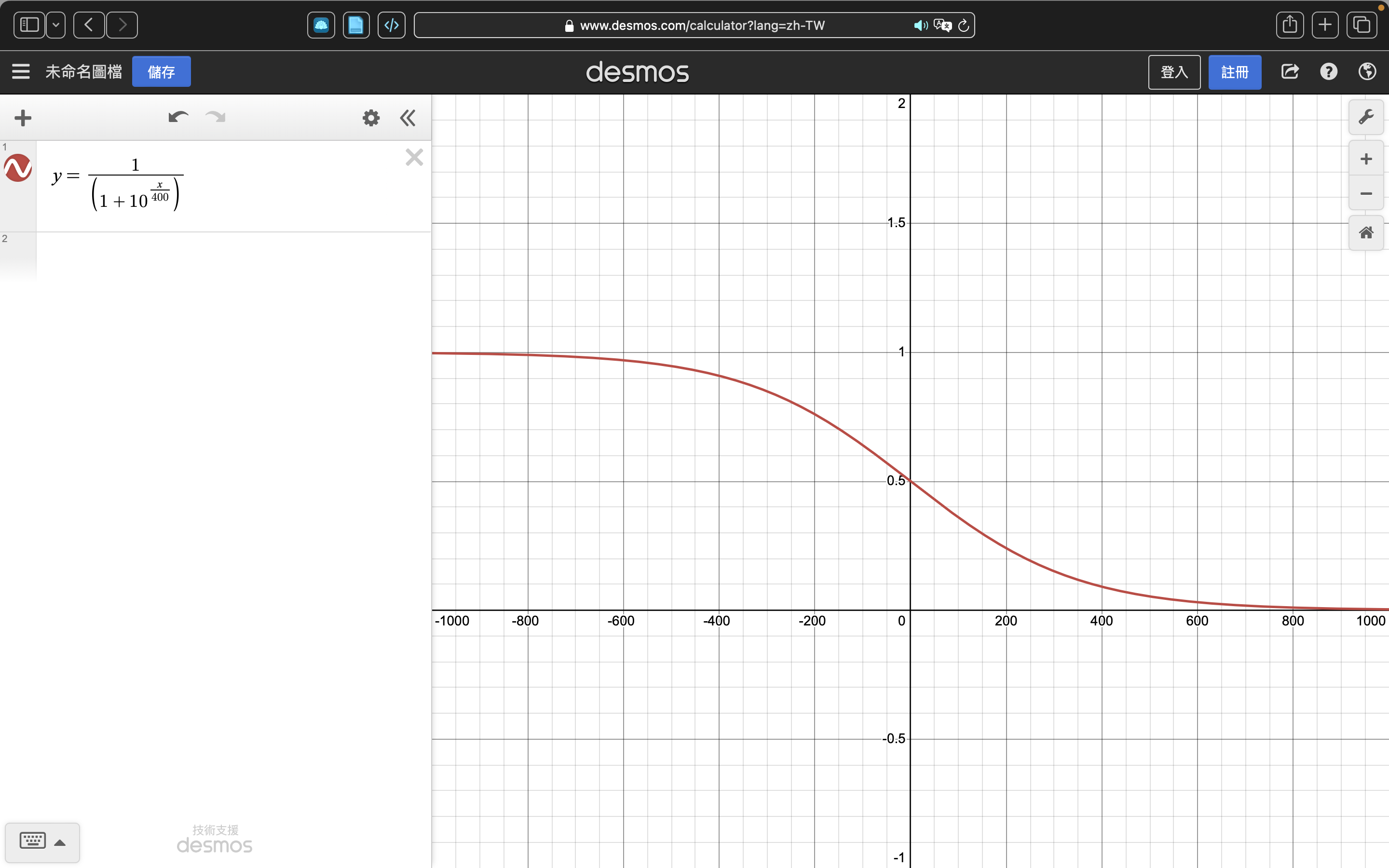
其實就是用分差把預期分數約束到0到1之間，其中勝利是1，失敗是0。

假設玩家A（當前分數$R_A$）的預期分數是$E_A$但是實際得分是$S_A$，玩家更新分數的公式是 $R_{\mathrm{A}}^{\prime}=R_{\mathrm{A}}+K \cdot\left(S_{\mathrm{A}}-E_{\mathrm{A}}\right).$

K-factor set at K=16 for masters and K=32 for weaker players.

Moreover, online judge sites are also using Elo rating system or its derivatives. For example, Topcoder is using a modified version based on normal distribution, while Codeforces is using another version based on logistic distribution.

Formal derivation for win/loss games
The above expressions can be now formally derived by exploiting the link between the Elo rating and the stochastic gradient update in the logistic regression.有的用隨機梯度更新分數

Logistic/Sigmoid

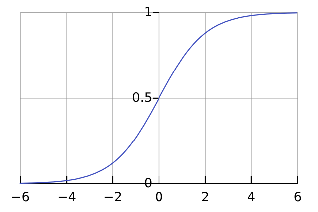
A logistic function or logistic curve is a common S-shaped curve (sigmoid curve) with the equation.

$f(x)=\frac{L}{1+e^{-k\left(x-x_0\right)}}$

where

• L is the carrying capacity, the supremum of the values of the function;
• k is the logistic growth rate, the steepness of the curve; and
• x0 is the x value of the function's midpoint. The logistic function has domain the real numbers, the limit as x→−∞ is 0, and the limit as x→+∞ is L.

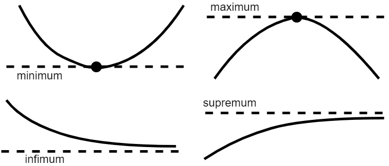
sup(X)是取上限函数，inf(X) 是取下限函数。 sup是supremum的简写，意思是：上确界，最小上界。 inf是infimum的简写，意思是：下确界，最大下界。

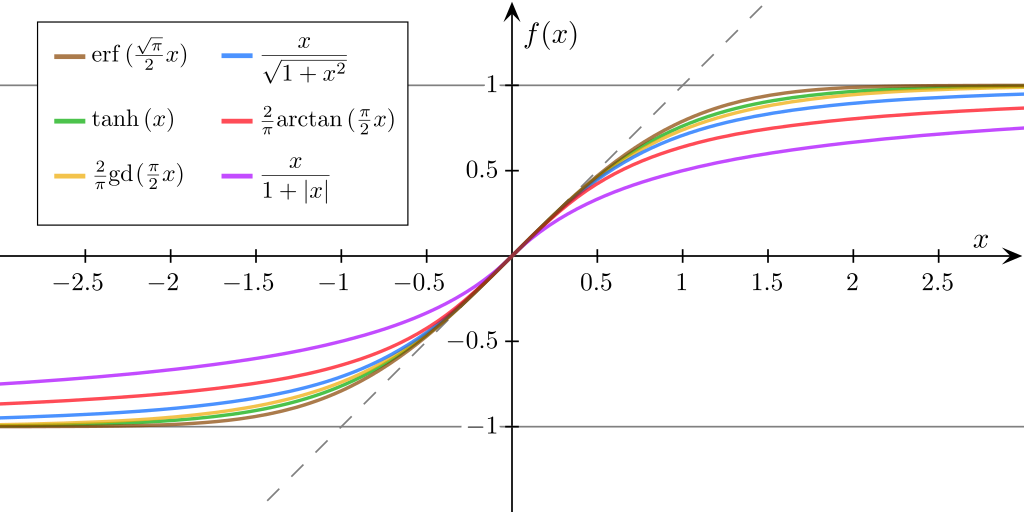
A sigmoid function refers specifically to a function whose graph follows the logistic function. It is defined by the formula:

$\sigma(x)=\frac{1}{1+e^{-x}}=\frac{e^x}{1+e^x}=1-\sigma(-x) .$

The logistic function was introduced in a series of three papers by Pierre François Verhulst between 1838 and 1847, who devised it as a model of population growth by adjusting the exponential growth model。

Exponential Growth：

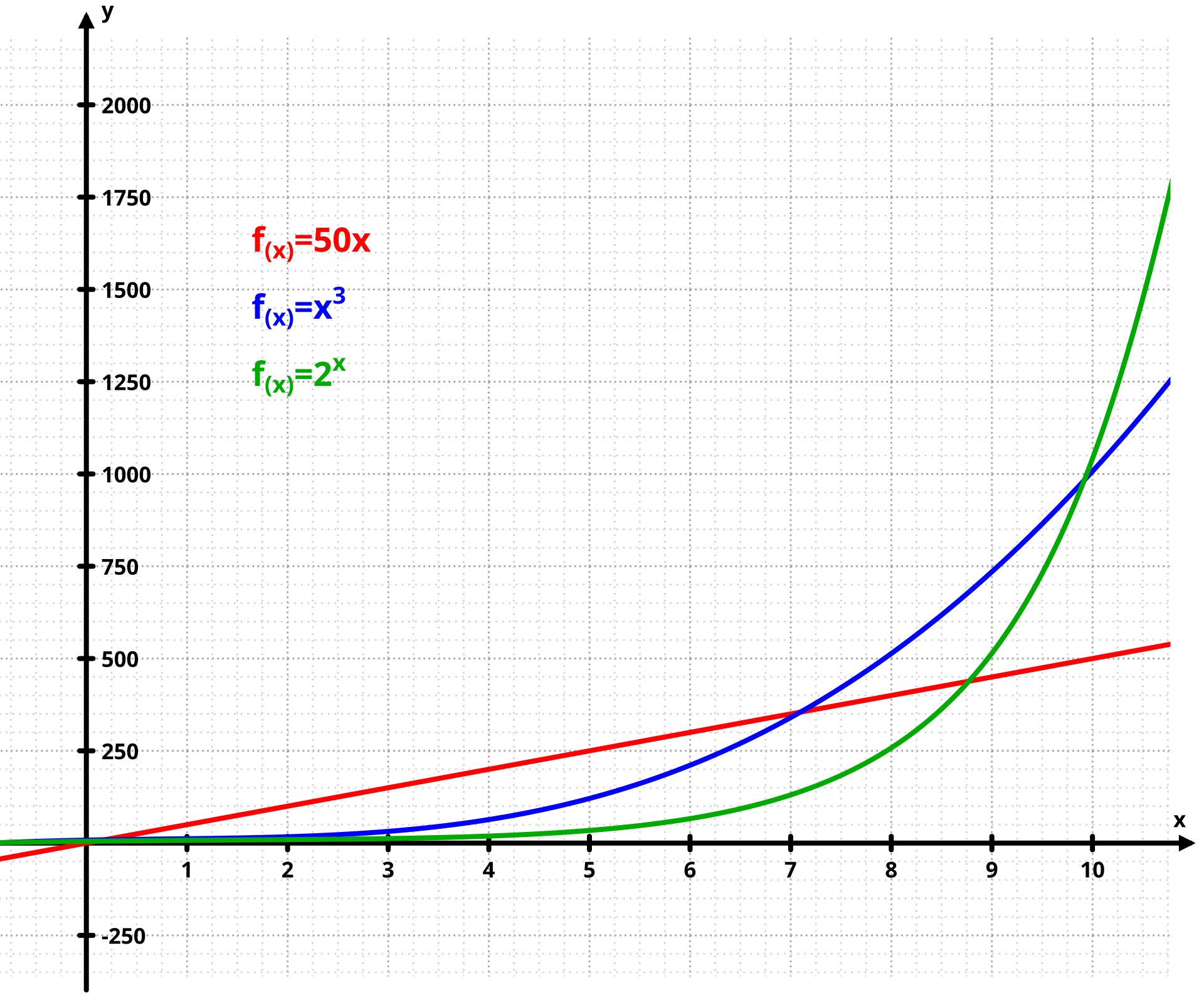
這logistic函數發明初衷是用於優化人口增長函數，在統計學和機器學習的應用只是它茫茫多應用的其中之一而已。
所有圖像長得像logsitic函數的都是sigmoid函數(S-shaped curve)。

Logistic functions are used in several roles in statistics. For example, they are the cumulative distribution function of the logistic family of distributions, and they are, a bit simplified, used to model the chance a chess player has to beat their opponent in the Elo rating system. More specific examples now follow.

Logistic regression

Logistic functions are used in logistic regression to model how the probability p of an event may be affected by one or more explanatory variables: an example would be to have the model

$p = f(a + bx),$

where x is the explanatory variable, a and b are model parameters to be fitted, and f is the standard logistic function.

Logistic regression and other log-linear models are also commonly used in machine learning. A generalisation of the logistic function to multiple inputs is the softmax activation function, used in multinomial logistic regression.

Log-linear

先複習一下，線性回歸是$y_i(x)=\beta_0+\beta_1x_i$，

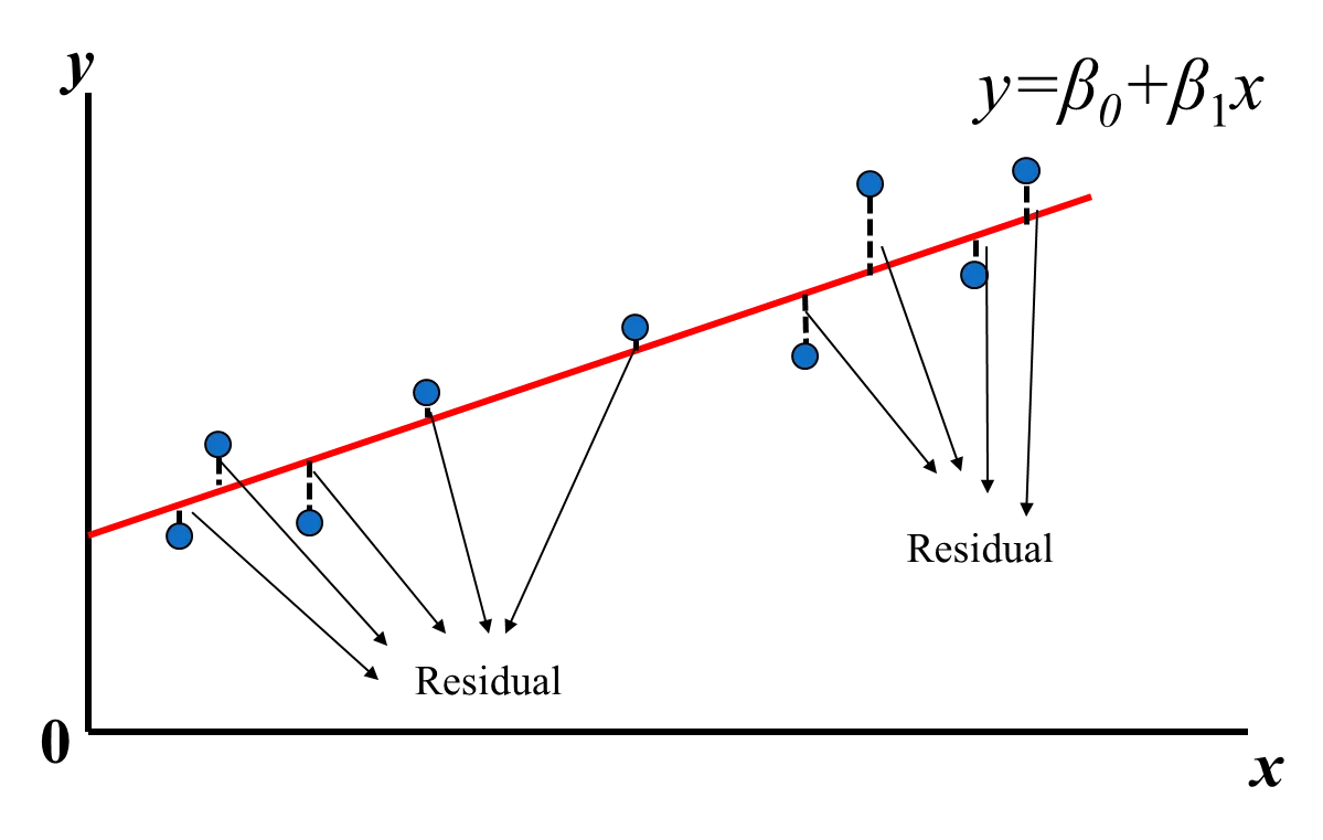
把數據$(x_i, y_i)$代入之後，用最小平方法(Least Square)計算loss function目標/損失函數， ${Loss}\left({\beta}_0, {\beta}_1\right)=\sum_{i=1}^n\left(y_i-\hat{y}_i\right)^2=\sum_{i=1}^n\left(y_i-\left({\beta}_0+{\beta}_1 x_i\right)\right)^2$ 之後更新beta修正函數擬合數據。

而log-linear就是把a+bx結果代入logistic或者其他sigmoid函數，好處是比如對分類任務來說，这个Sigmoid Function可以将线性的值，映射到[0-1]范围中。如果映射结果小于0.5，则认为是负的样本，如果是大于0.5，则认为是正的样本。

採用logistic分布和gaussian/normal分布的區別？

A workable rating system, fully developed from basic theory, includes certain principal components:

1. Rating scale
2. Performance distribution function
3. Percentage expectancy function
4. Performance rating formula
5. Continuous rating formula
6. Appropriate numerical coefficients and ancillary formulae —— 8.12 The Rating of Chessplayers, Past & Present, Second Edition, Arpad E. Elo

區別就是預期分數（player's expected score）的計算公式，上面用的logistic function(base10)其實就是logistic distribution的CDF，可以發現如下圖所示跟normal distribution的CDF很像。

• In probability theory and statistics, the logistic distribution is a continuous probability distribution.
• Its cumulative distribution function is the logistic function, which appears in logistic regression and feedforward neural networks.
• It resembles the normal distribution in shape but has heavier tails (higher kurtosis).

logistic distribution其實就是尾部更長的normal distribution了。

Logistic distribution				Normal distribution
Probability density function	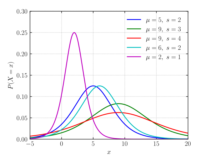			Probability density function 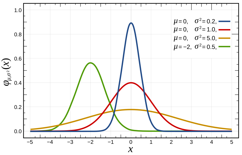The red curve is the standard normal distribution.
Cumulative distribution function	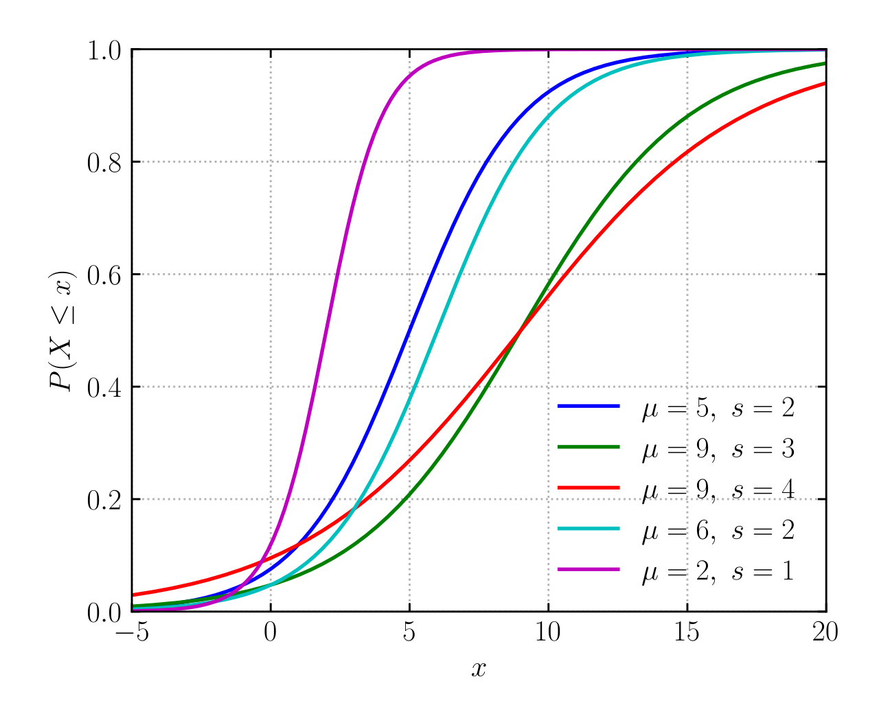			Cumulative distribution function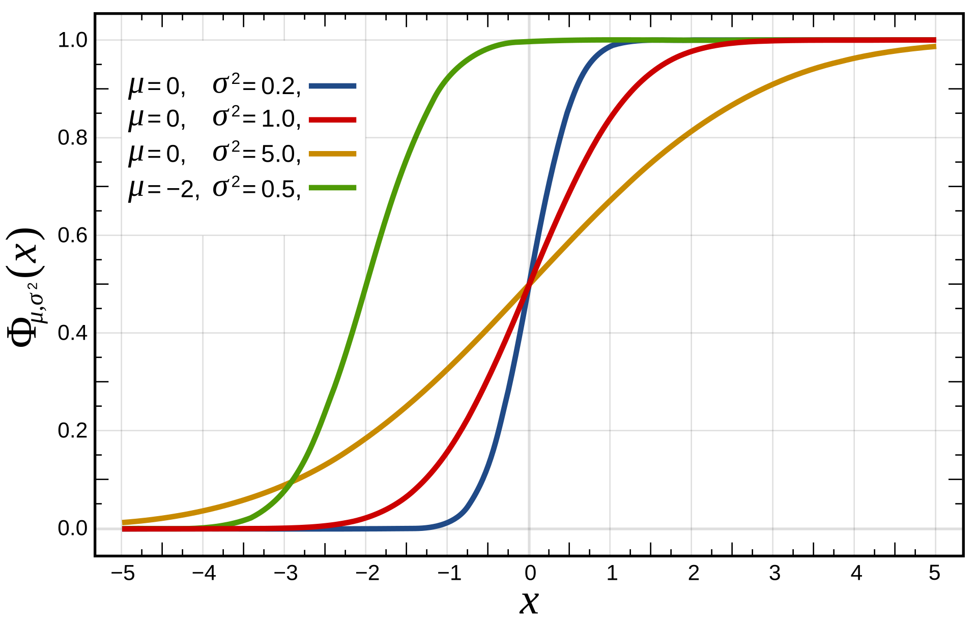
Notation	LogisticDistribution(μ,s)			${\displaystyle {\mathcal {N}}(\mu ,\sigma ^{2})}$
Parameters	${\displaystyle \mu ,}$ location (real) ${\displaystyle s>0,}$ scale (real)			${\displaystyle \mu \in \mathbb {R} }$ = mean (location) ${\displaystyle \sigma ^{2}\in \mathbb {R} _{>0}}$ = variance (squared scale)
Support	${\displaystyle x\in (-\infty ,\infty )}$			${\displaystyle x\in \mathbb {R} }$
PDF	${\displaystyle {\frac {e^{-(x-\mu )/s}}{s\left(1+e^{-(x-\mu )/s}\right)^{2}}}}$			${\displaystyle {\frac {1}{\sqrt {2\pi \sigma ^{2}}}}e^{-{\frac {(x-\mu )^{2}}{2\sigma ^{2}}}}}$
CDF	${\displaystyle {\frac {1}{1+e^{-(x-\mu )/s}}}={\frac {1+\tanh {\frac {x-\mu }{2s}}}{2}}}$			${\displaystyle \Phi \left({\frac {x-\mu }{\sigma }}\right)={\frac {1}{2}}\left[1+\operatorname {erf} \left({\frac {x-\mu }{\sigma {\sqrt {2}}}}\right)\right]}$
Quantile	${\displaystyle \mu +s\log \left({\frac {p}{1-p}}\right)}$			${\displaystyle \mu +\sigma {\sqrt {2}}\operatorname {erf} ^{-1}(2p-1)}$
Mean	${\displaystyle \mu }$			${\displaystyle \mu }$
Median	${\displaystyle \mu }$			${\displaystyle \mu }$
Mode	${\displaystyle \mu }$			${\displaystyle \mu }$
Variance	${\displaystyle {\frac {s^{2}\pi ^{2}}{3}}}$			${\displaystyle \sigma ^{2}}$

Probability theory basics機率基礎

https://www.youtube.com/watch?v=GwSEguqJj6U&list=PLtvno3VRDR_jMAJcNY1n4pnP5kXtPOmVk
台大電機 Prof. 葉丙成 機率與統計 2013，這個講得超好。

為什麼我們要研究機率？
因為我們對這世界了解太少，這世界的運作有很多仍是未知的。——prof.benson

術語：

• Experiment實驗(procedures實驗步驟、model機率模型、observations結果觀察，三個部分任何一個改變，都會變為新的實驗)，
• Outcome結果，
• Sample Space樣本空間，若是S={o1,...,on}n個outcome的集合
• Event事件（實驗結果的敘述，因此是Outcome的集合，或者是Sample Space的子集），
• Event Space事件空間，則為{{o1},...,{on},{o1,o2},{o1,o3},...,{on-1,on},{o1,o2,o3},...,{o1,o2,...,on},{}}一共2^n個事件元素的集合
• Probability機率（是個函數，P(Event)，Probability is a function of Event(Set)，Domain定義域就是Event Space，Range值域是[0,1]）
• Set Theory（因為Probability is a function of Set，所以要了解Set）術語：
  • Element, Set, Subset, Universal Set全集, Empty Set, Intersection交集, Union并集/聯集, Complement補集, Difference差集(X - Y), Disjoint不相交(X, Y disjoint if X∩Y=∅), Mutually Exclusive互斥（兩個set是disjoint，一堆集合兩兩不相交就是互斥）
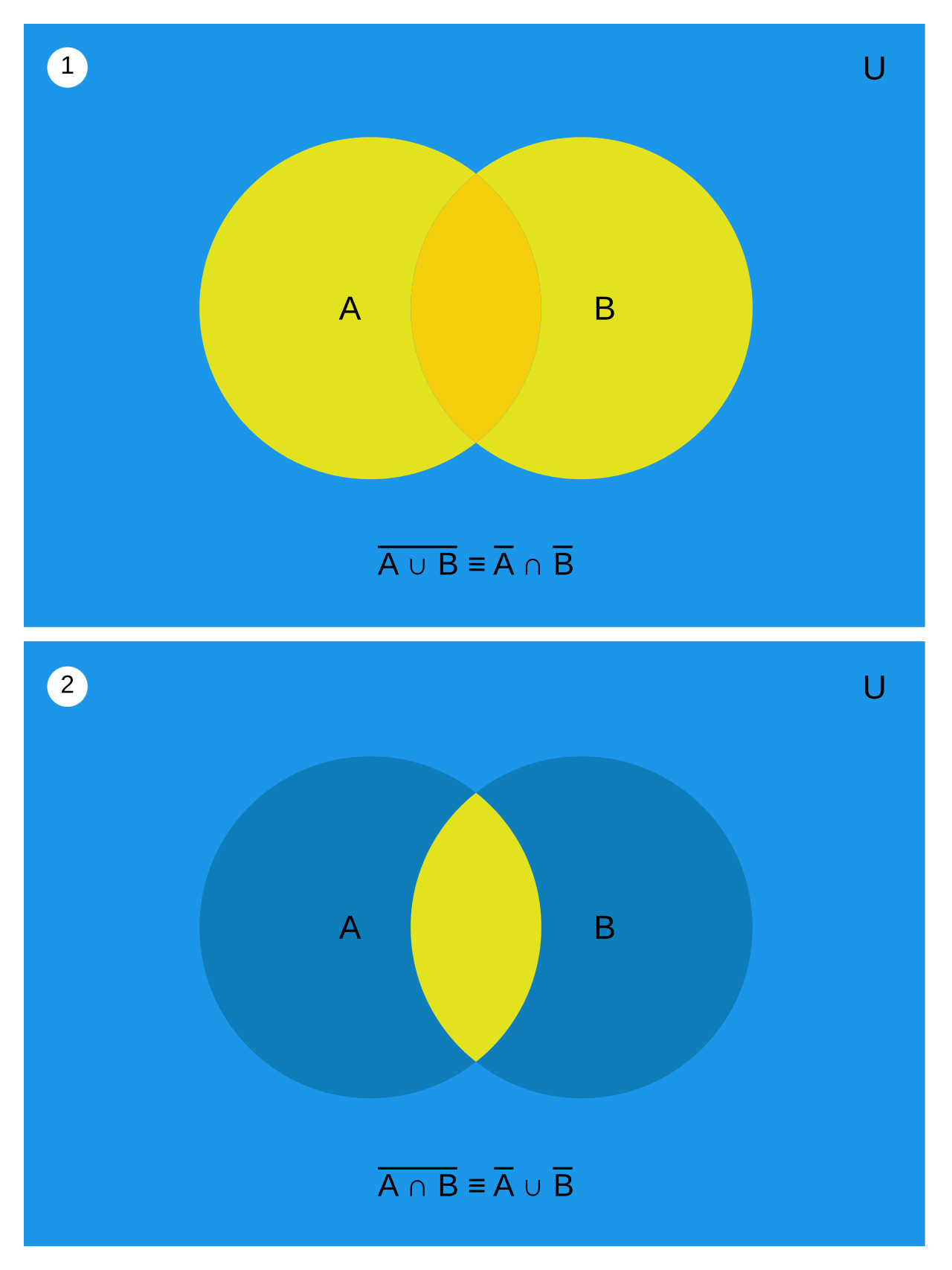
  • De Morgan's Law:

為什麼事件空間是2^n？一次實驗裡兩個結果，三個結果怎麼可能同時發生？
剛開始這個疑問就是沒搞清結果和事件的區別，一個事件可能包含多個結果。（37分鐘有例子）

Axioms /ˈaksɪəm/

從這部影片第一次了解一個理論的公理，中國大陸的教學真差。 近代數學常從數條公理推導出整套理論，線性代數有8(9?)條公理(9 axioms of linear algebra/real vector spaces):

• Additive axioms. For every x,y,z in X, we have
  • x+y = y+x.
  • (x+y)+z = x+(y+z).
  • 0+x = x+0 = x.
  • (-x) + x = x + (-x) = 0.
• Multiplicative axioms. For every x in X and real numbers c,d, we have
  • 0x = 0
  • 1x = x
  • (cd)x = c(dx)
• Distributive axioms. For every x,y in X and real numbers c,d, we have
  • c(x+y) = cx + cy.
  • (c+d)x = cx +dx. 整套理論只基於幾條公理的好處是，對於一個新問題只需要確定滿足這些公理（其實沒有定義“+”要怎麼做，是general的，套別的case其實不一定滿足），就能適用其他所有定理。 公理不用證明，axioms是理性直覺覺得是對的東西。只從這幾條廢話推導出所有定理確實牛逼。

Axioms of Probability(機率三公理):

• Axiom 1: For any event A, $P(A) \geq 0$
• Axiom 2: Probability of the sample space S is $P(S)=1$
• Axiom 3: If A1,A2,A3,⋯ are disjoint events, then $P(A_1 \cup A_2 \cup A_3 \cdots)=P(A_1)+P(A_2)+P(A_3)+\cdots$

axiom3的disjoint即互斥。

性質(定理)

• P(A) = P(A-B) + P(A∩B)
• P(A∪B) = P(A) + P(B) - P(A∩B)
• 切麵包定理：若 $C_1, C_2, \cdots, C_n$互斥，且$C_1 \cup C_2 \cup \cdots \cup C_n = S$，則对任何事件 A：$P(A) = P(A \cap C_1) + P(A \cap C_2) + \cdots + (A \cap C_n)$
• 若A⊂B則P(A)≤P(B)
• Boole's inequality/Union Bound布爾不等式：對任何事件A1, A2, ..., An，$\mathbb{P}\left(\bigcup_i A_i\right)\leq \sum_i\mathbb P(A_i)$
• Bonferroni's inequality

conditional probability條件機率(貝氏定理)

P ( X | Y ), Y是觀察到的已發生的事件，X是關心的未發生的事件。

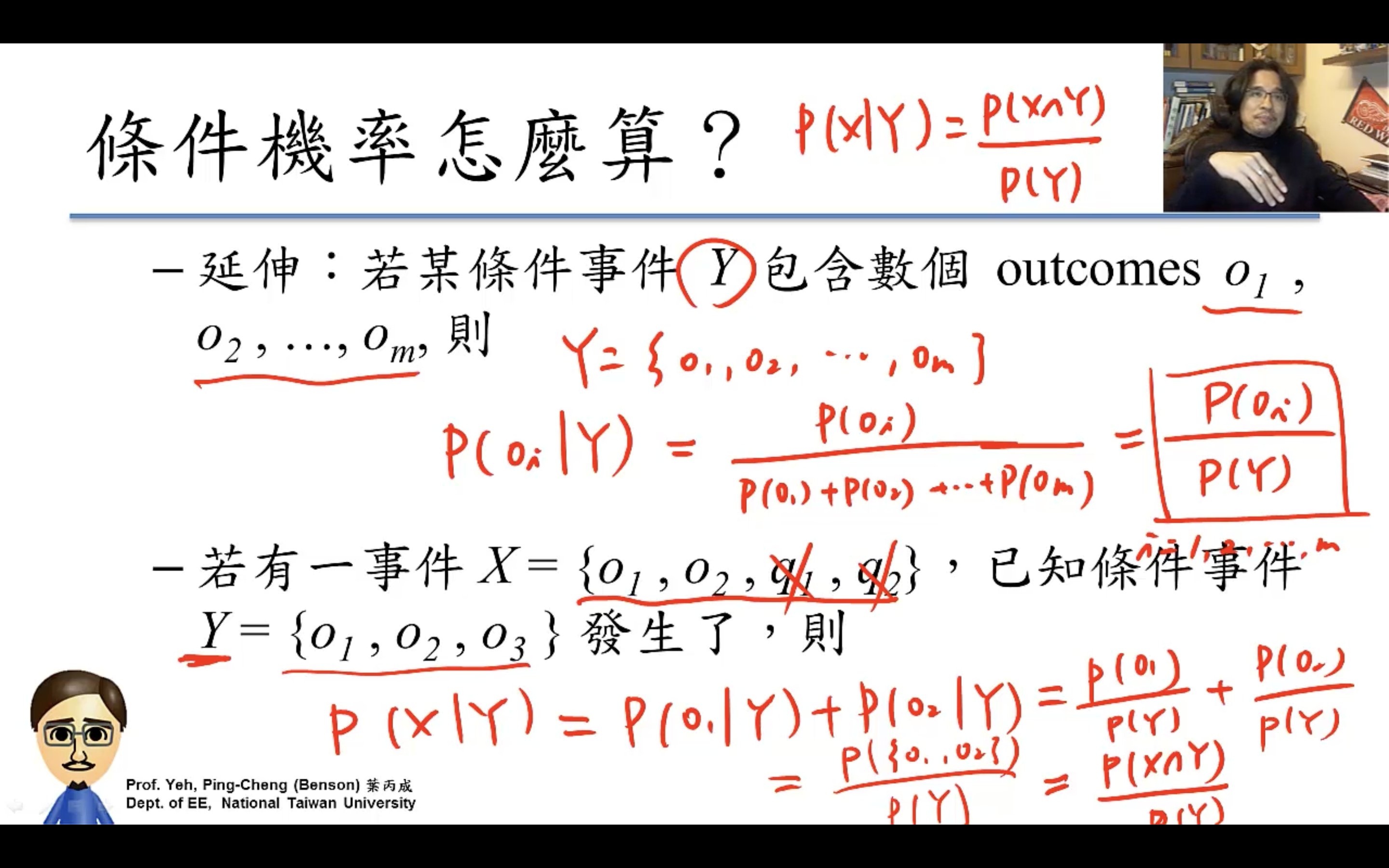
tex公式裡∪是\cup，∩是\cap，一個杯子一個帽子很形象很有趣。

$P(X|Y) = \frac{P(X\cap Y)}{P(Y)}$

P ( X | Y )可以理解成只是樣本空間S變成了Y而已。

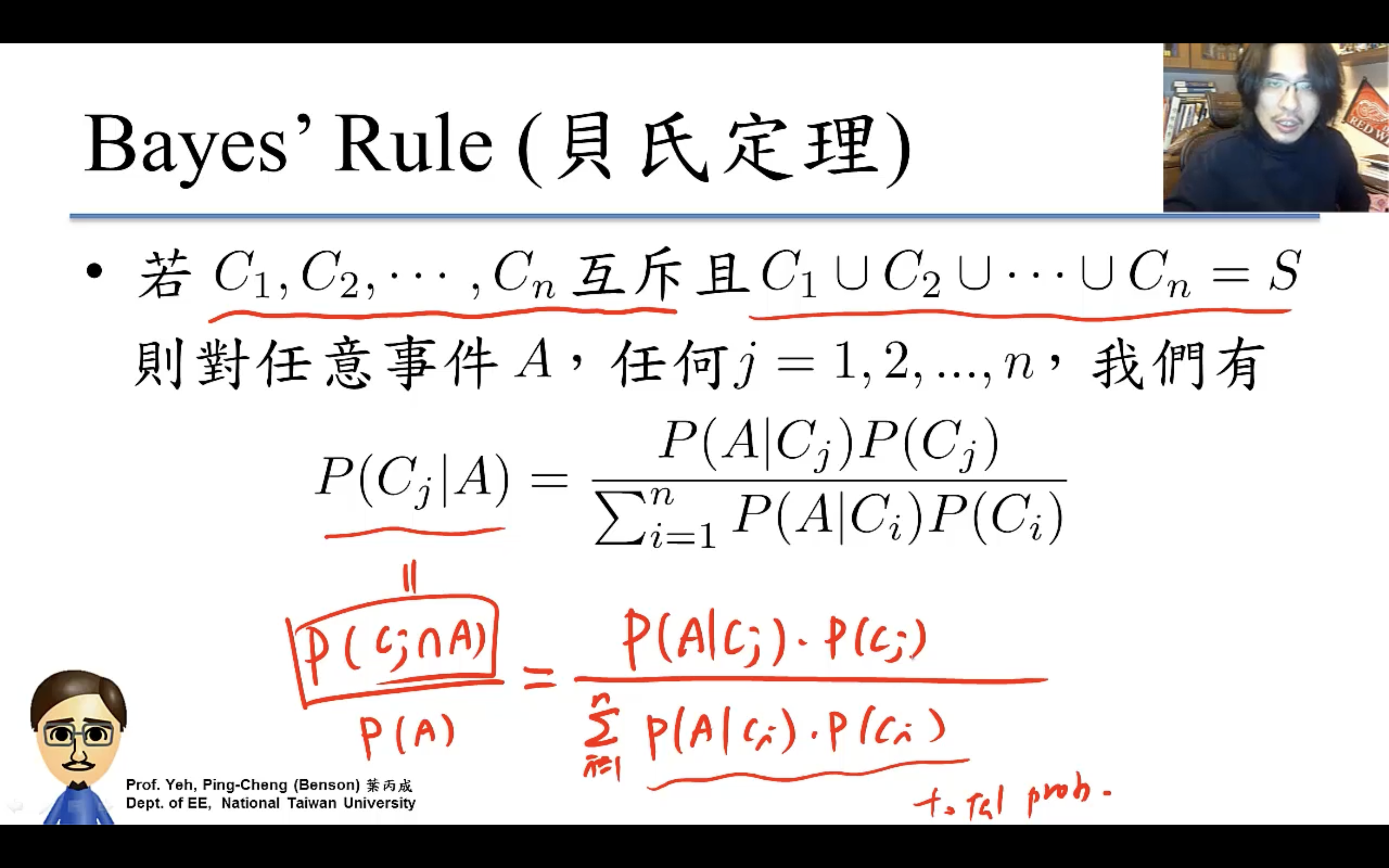
若事件C1, C2 . . . Cn互斥且S = C1 ∪ C2 ∪ . . . . . ∪ Cn，則對任意事件A，

• Law of Total Probability(切麵包)，$\begin{array}{l} P(A) =\sum\limits_{i=1}^{n} P(C_i)P(A| C_i)\end{array}$。Ex：阿宅 vs. 可愛店員：店員對阿宅笑否，受店的生意影響很大。已知滿座機率，可愛店員對阿宅笑的機率？
• Bayes' Rule, $P(C_j|A)=\frac{P(A|C_j)P(C_j)}{\sum\limits_{i=1}^{n} P(A | C_i) P(C_i)}$，之前算的都是P of A given C，貝葉斯是解決計算P of C given A。Ex：一日，老闆見可愛店員笑，請問在此情況下，當日生意滿座之機率為何？
  

Independence(獨立性)

若滿足P(A∩B)=P(A)P(B)則A、B兩事件為獨立事件。
跟互斥對比：A∩B=∅不可能事件即P(A∩B)=0。

可以理解成兩個實驗的樣本空間沒有交集？

Prof. Benson立刻就講到了更好的定義，若滿足P(A|B) = P(A)則A、B兩事件為獨立事件。

根據上面的理解“P ( X | Y )可以理解成只是樣本空間S變成了Y而已”，即Y的樣本空間跟X完全沒有關係，比如X的樣本空間是{o1, o2, ..., on}，Y的樣本空間是{p1, p2, ..., pn}，事件Y可能是{p1, p2, p3}，完全不影響這個世界裡事件X發生與否，這裡的Y實際上是{p1, p2, p3, o1, o2, ..., on}。

非獨立事件的conditional probability是這樣的：假如實驗是投一個6面骰子一次，樣本空間是{1,2,3,4,5,6}，X事件是扔出{1,5,6}，Y事件是扔出大數{4,5,6}，那X｜Y的樣本空間就變成了{4,5,6}即X只可能是扔出了大數中的某個數，o1∩Y=∅，X就變成{5,6}，P(X｜Y)則=P({5,6})/P({4,5,6})=2/3。

Graph Scheme

實驗分解。

counting method

為什麼機率需要算排列組合，需要counting？
因為古典機率常假設每個outcome發生機率相同，所以計算某個事件的機率，等同於計算這個事件包含多少個outcome，像上面計算事件空間那樣，機率（事件）=outcome數/事件空間元素數。所以機率問題等於counting問題。

counting前的判斷：

• distinguishable? 可區分？
• w/wo replacement? 有放回？
• order matters or not? 關心順序嗎？if order matters then Permutation (排列問題) else Combination (組合問題)

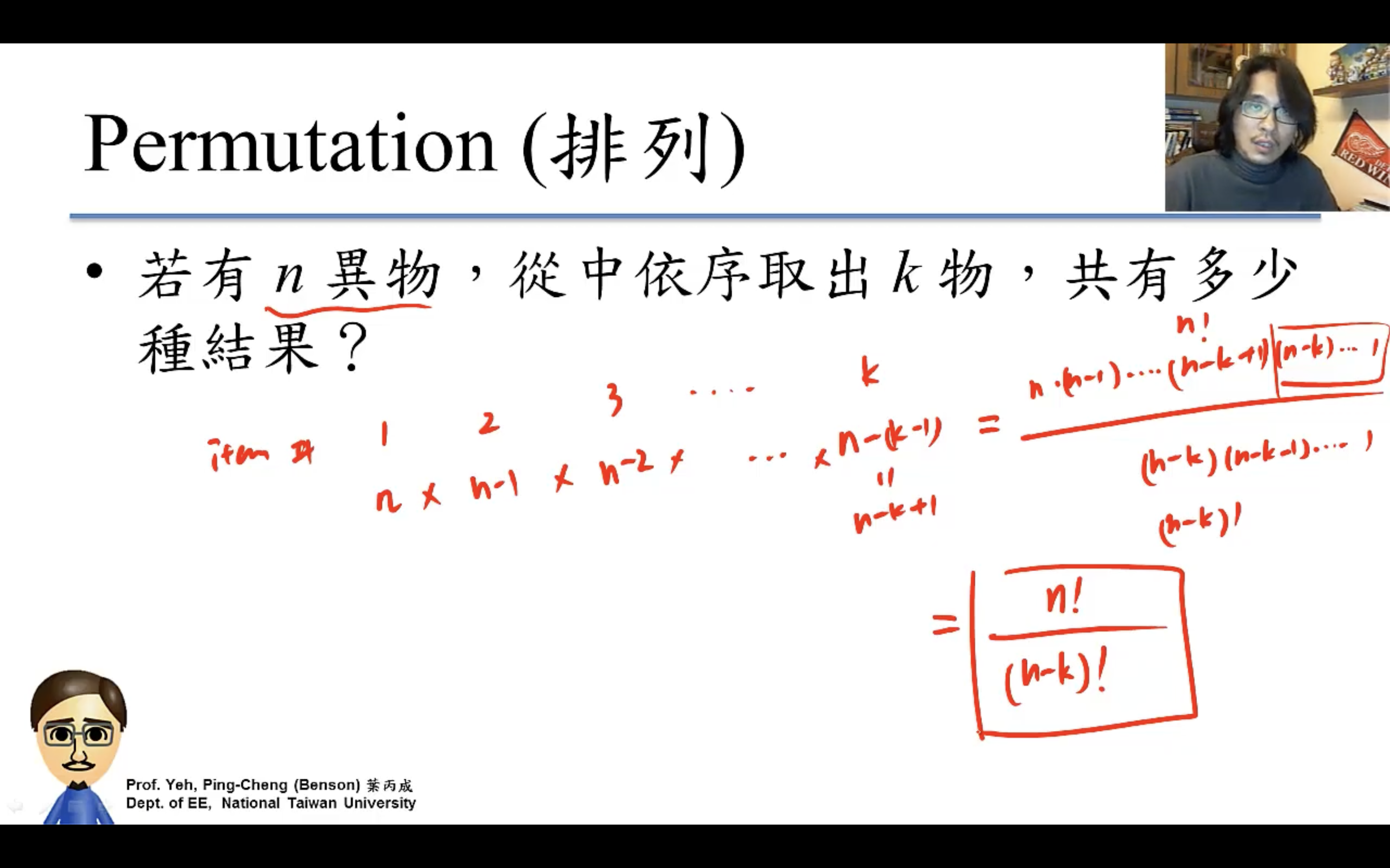
Permutation(order matters)

• w/o replacement
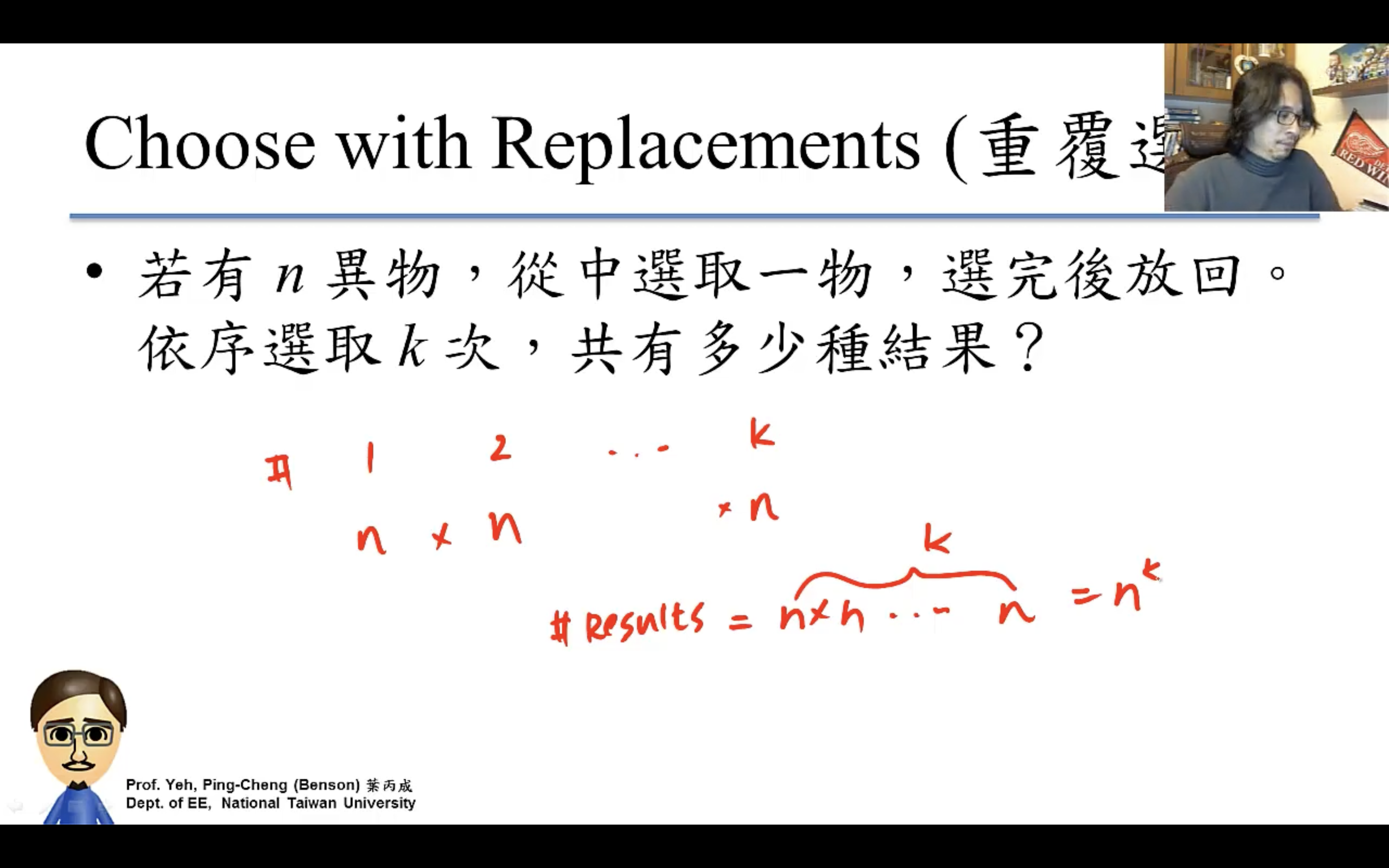
• w/ replacement

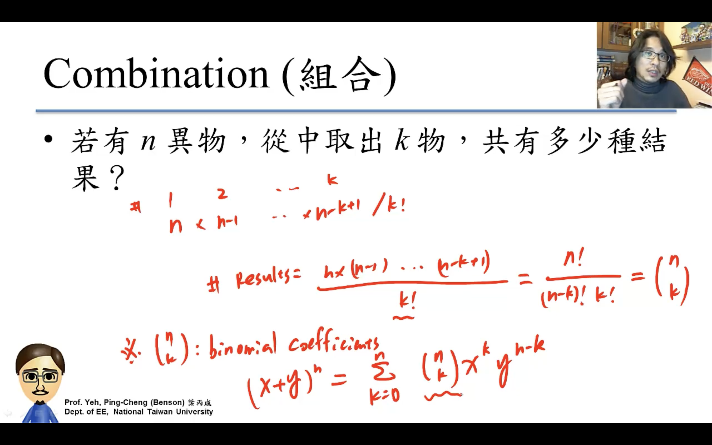
Combination(order doesn't matter)

除以k!就是因為order doesn't matter，要把order的排列除掉，也就是k個items的所有排列方式k!種（比如3個items有6種排列方式=3!）。

數學裡叫n choose k，n取k。

$C(n, k) = \binom{n}{k} = C_n^k = \frac{n!}{k!(n-k)!}$

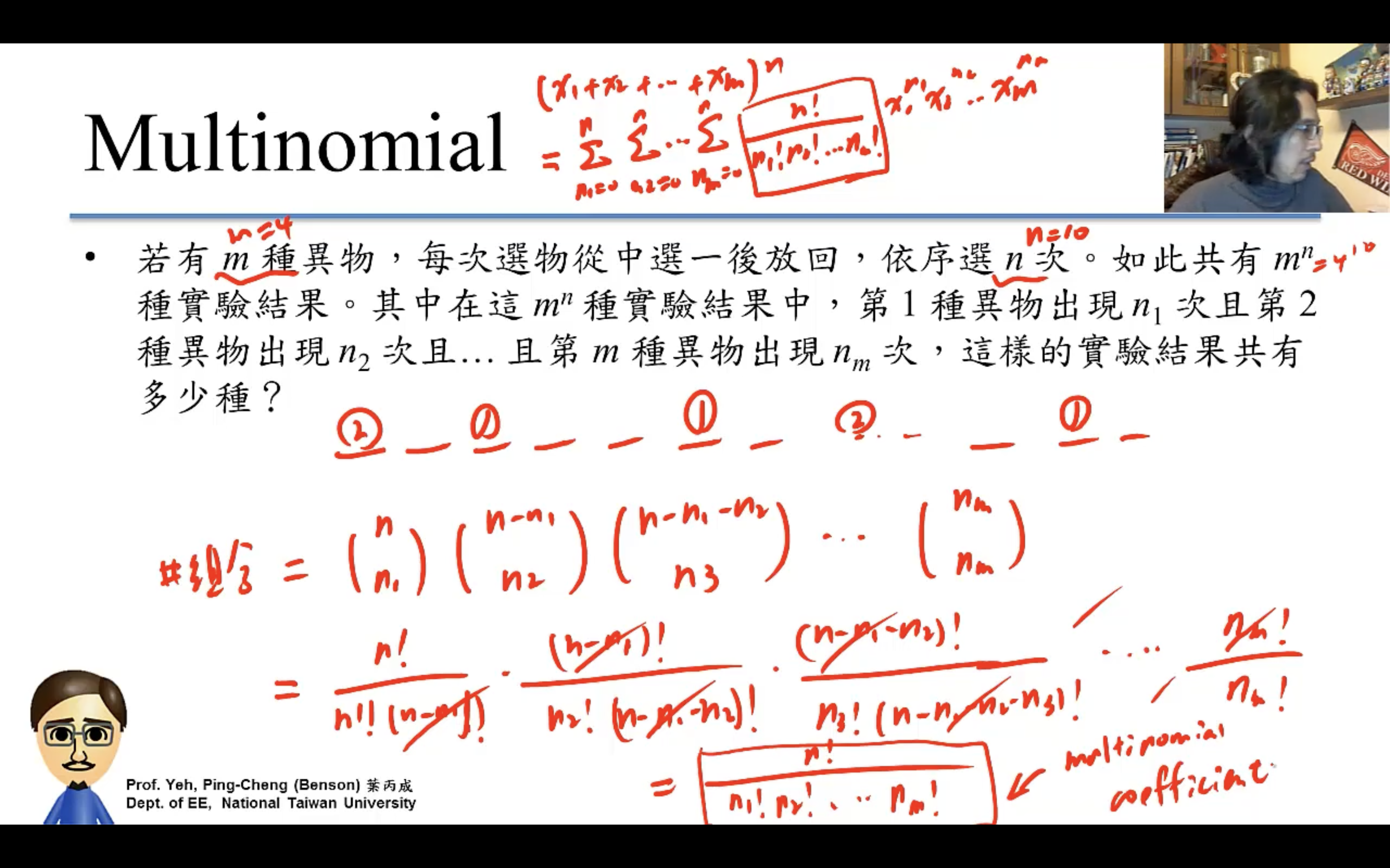
Multinomial

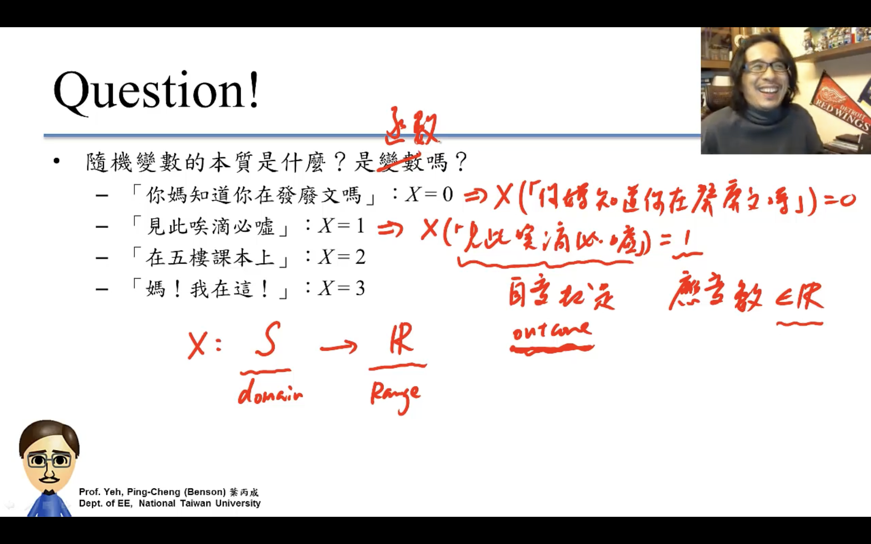
Random Variable隨機變數

就是把outcome數字化的方式，讓推導更數學、更簡明。

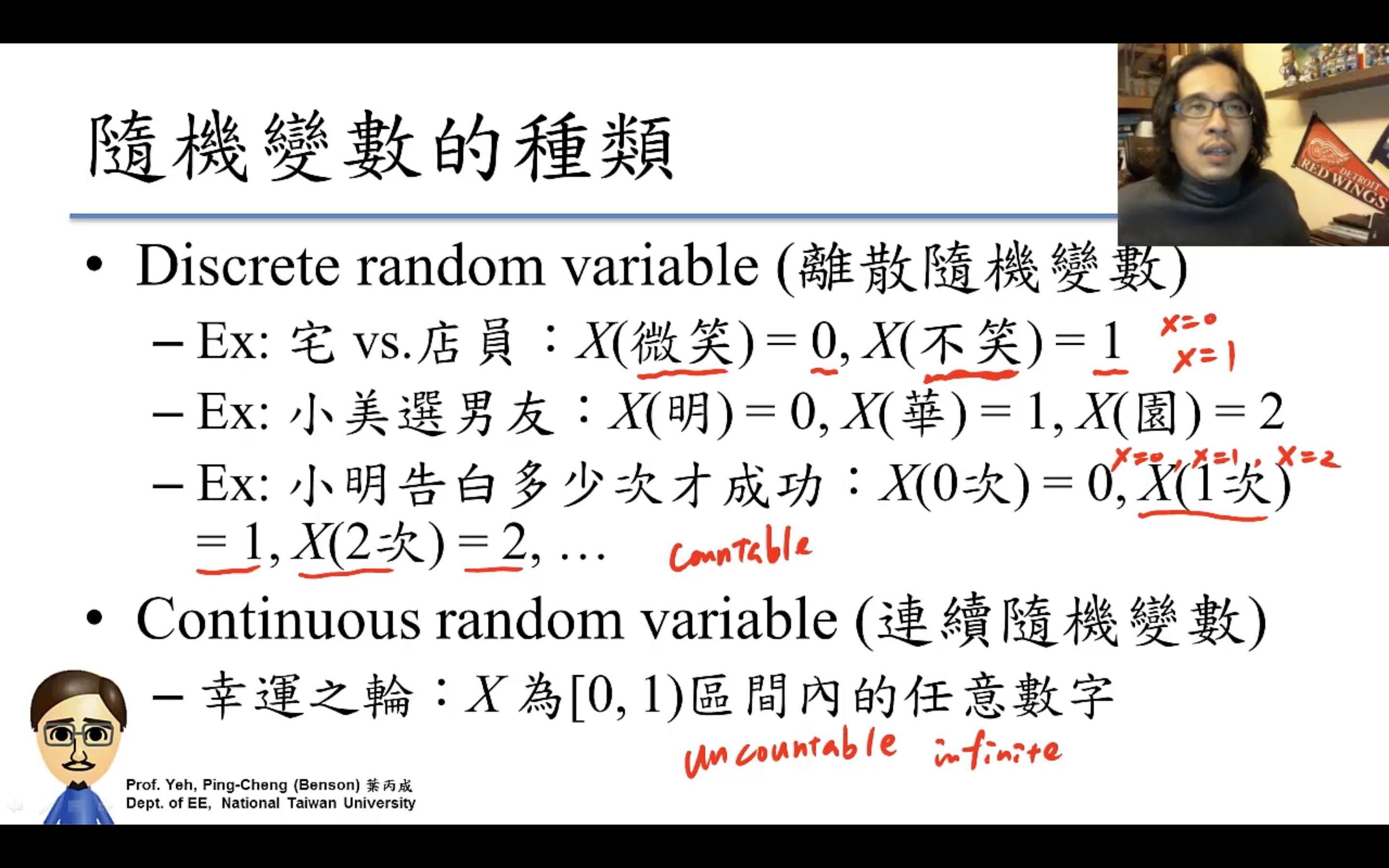
• Discrete R.V. (離散隨機變數)
• Continuous R.V. (連續隨機變數)

隨機變數的函數也是隨機變數，因為outcome的函數的函數也是outcome的函數。

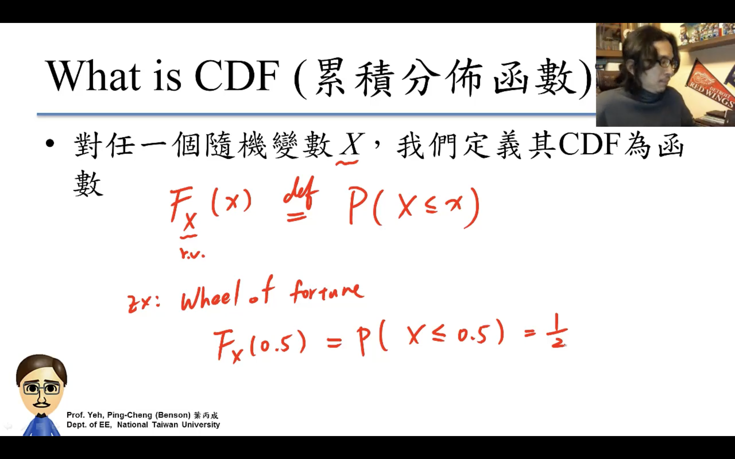
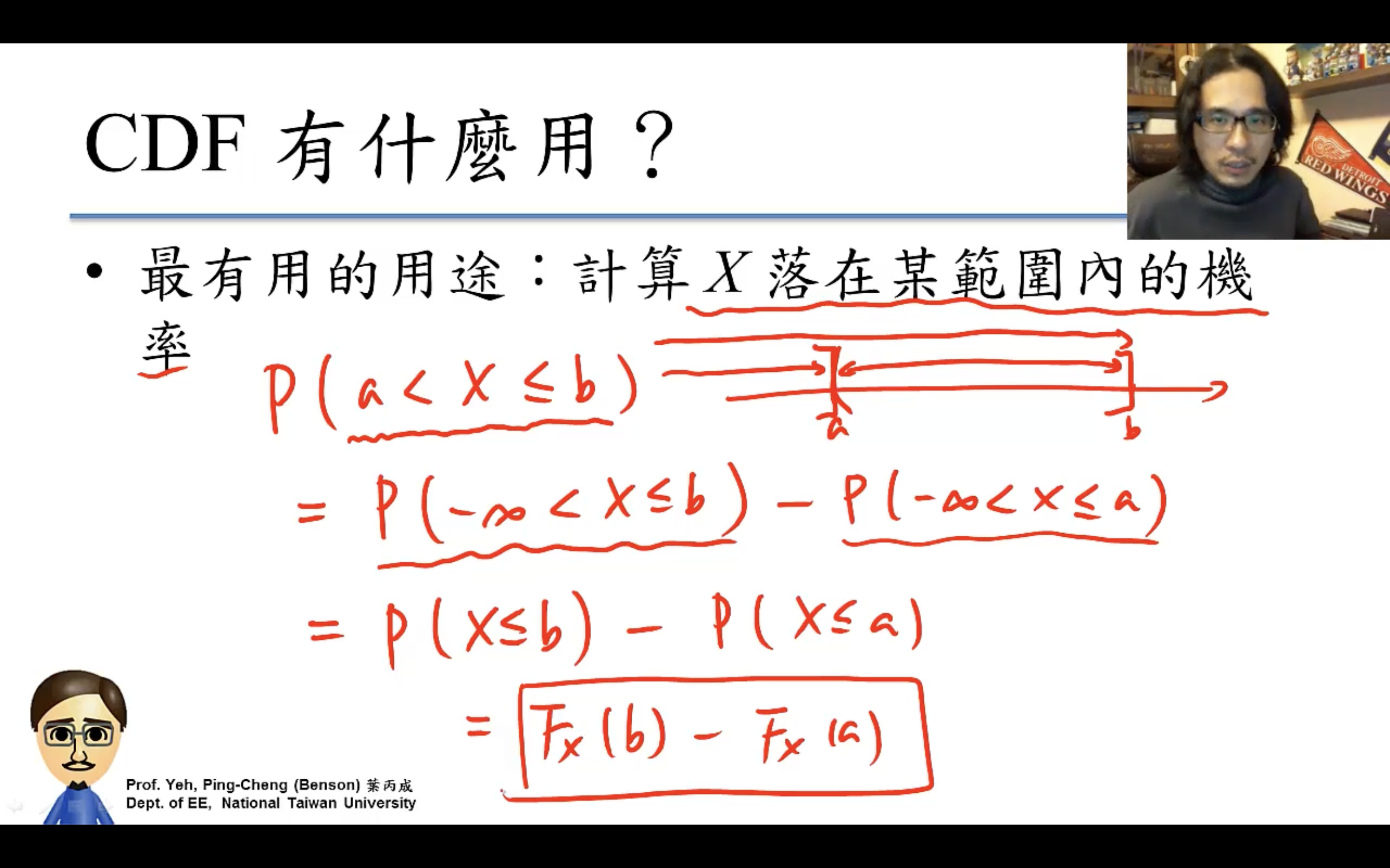
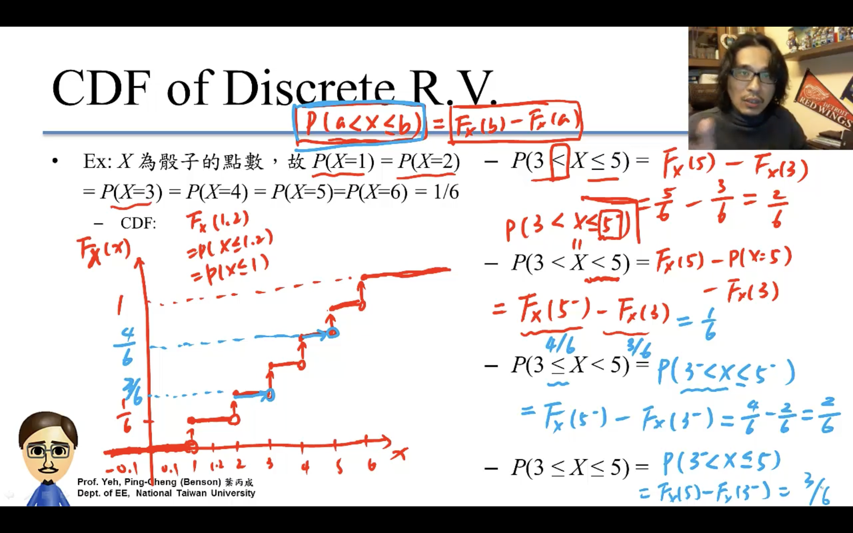
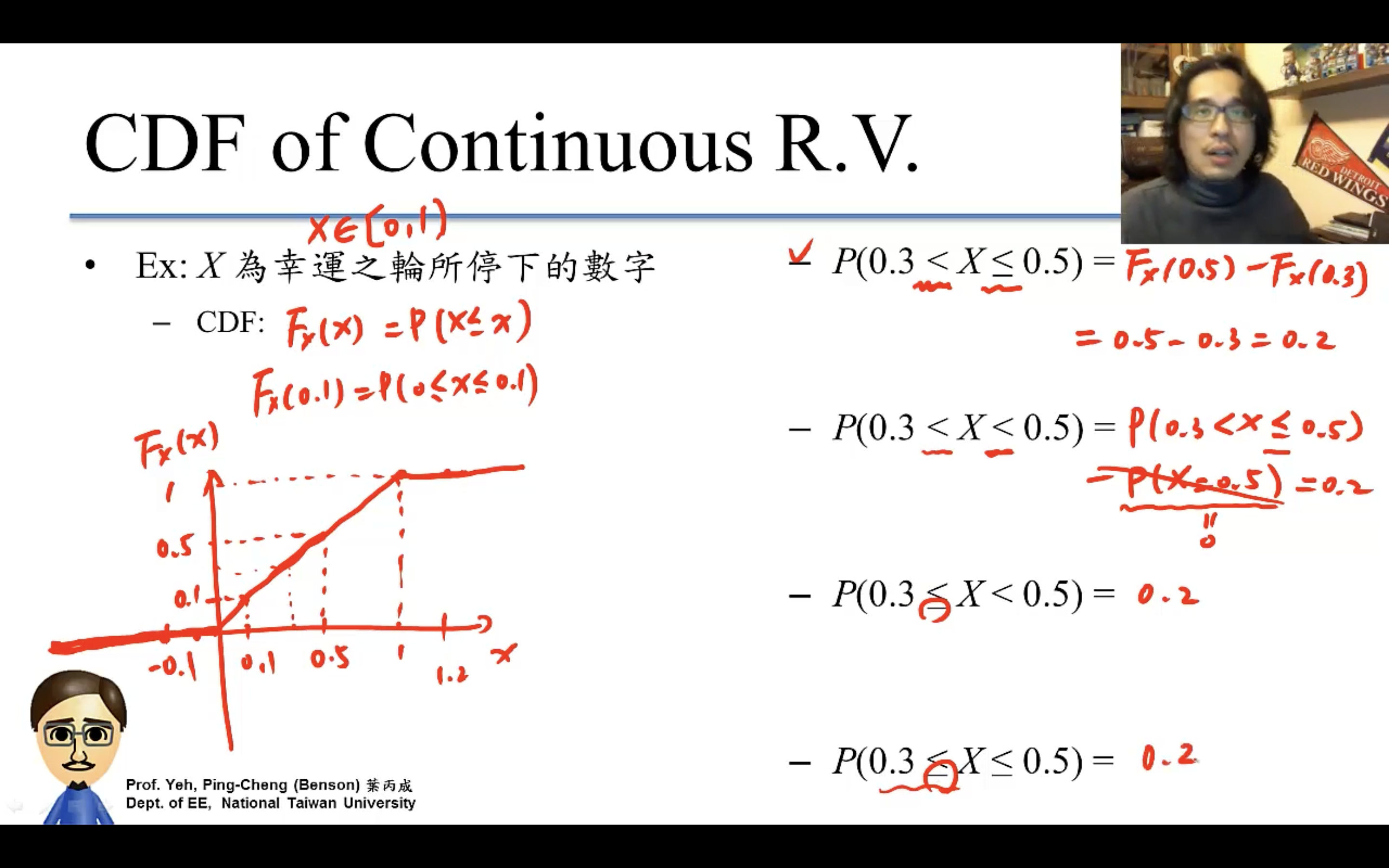
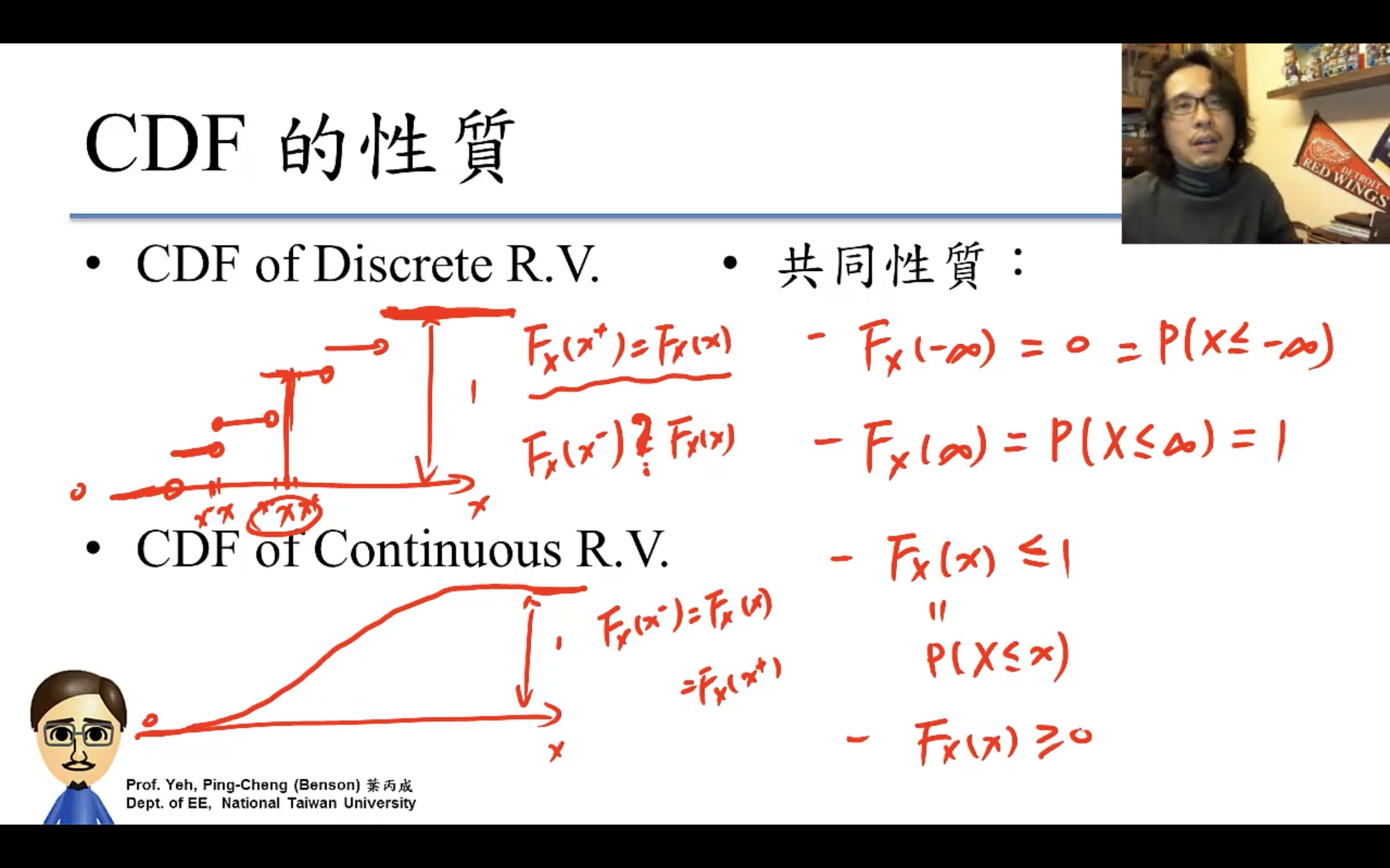
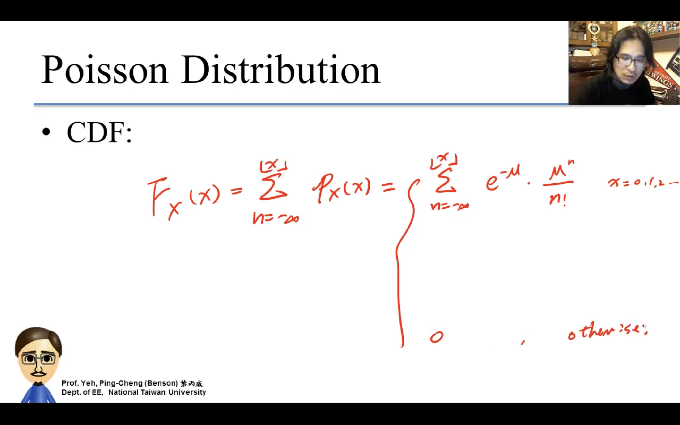
CDF (Cumulative Distribution Function)

累計分佈函數$F_X(x) = P(X \le x)$。

PMF (Probability Mass Function)

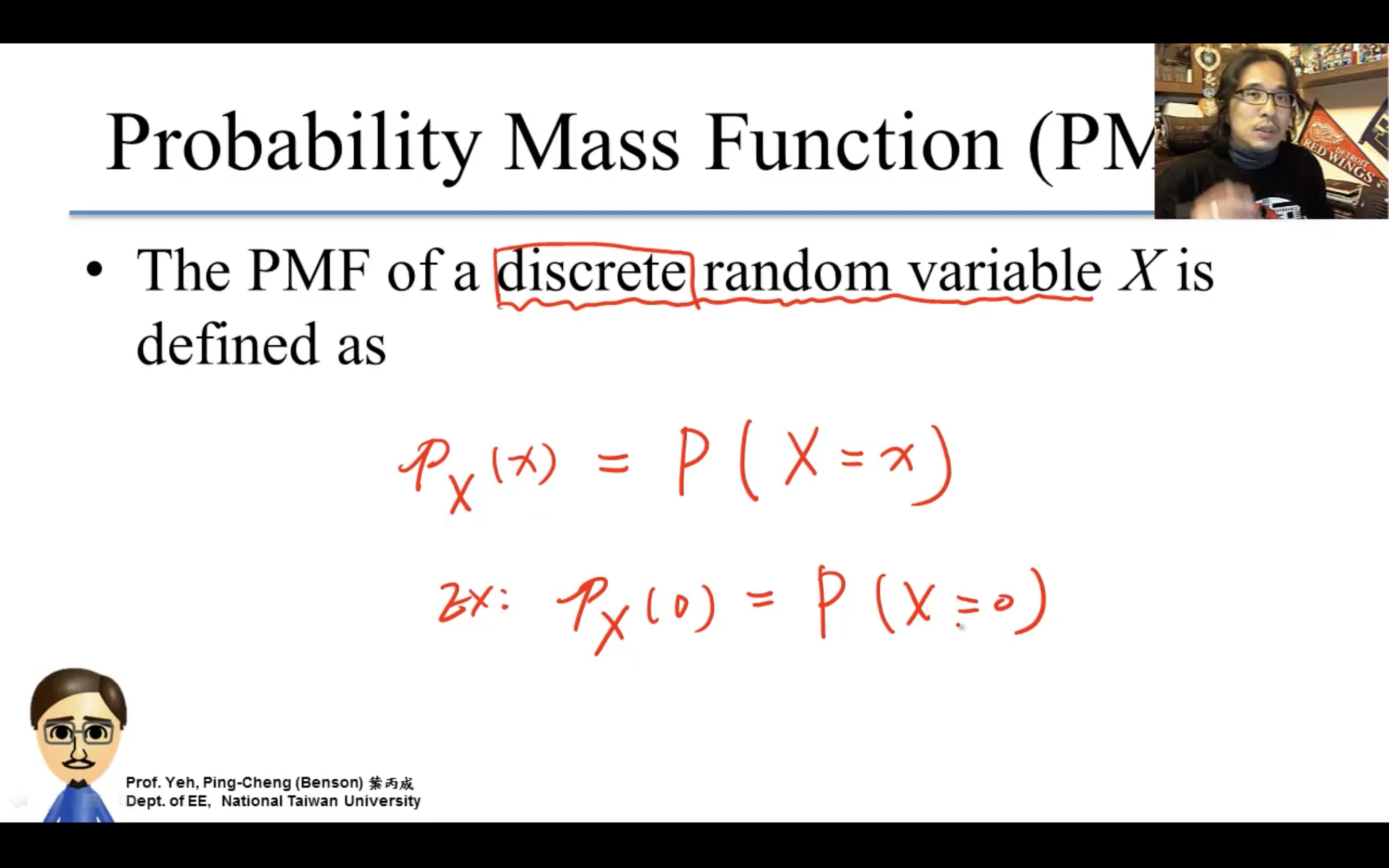
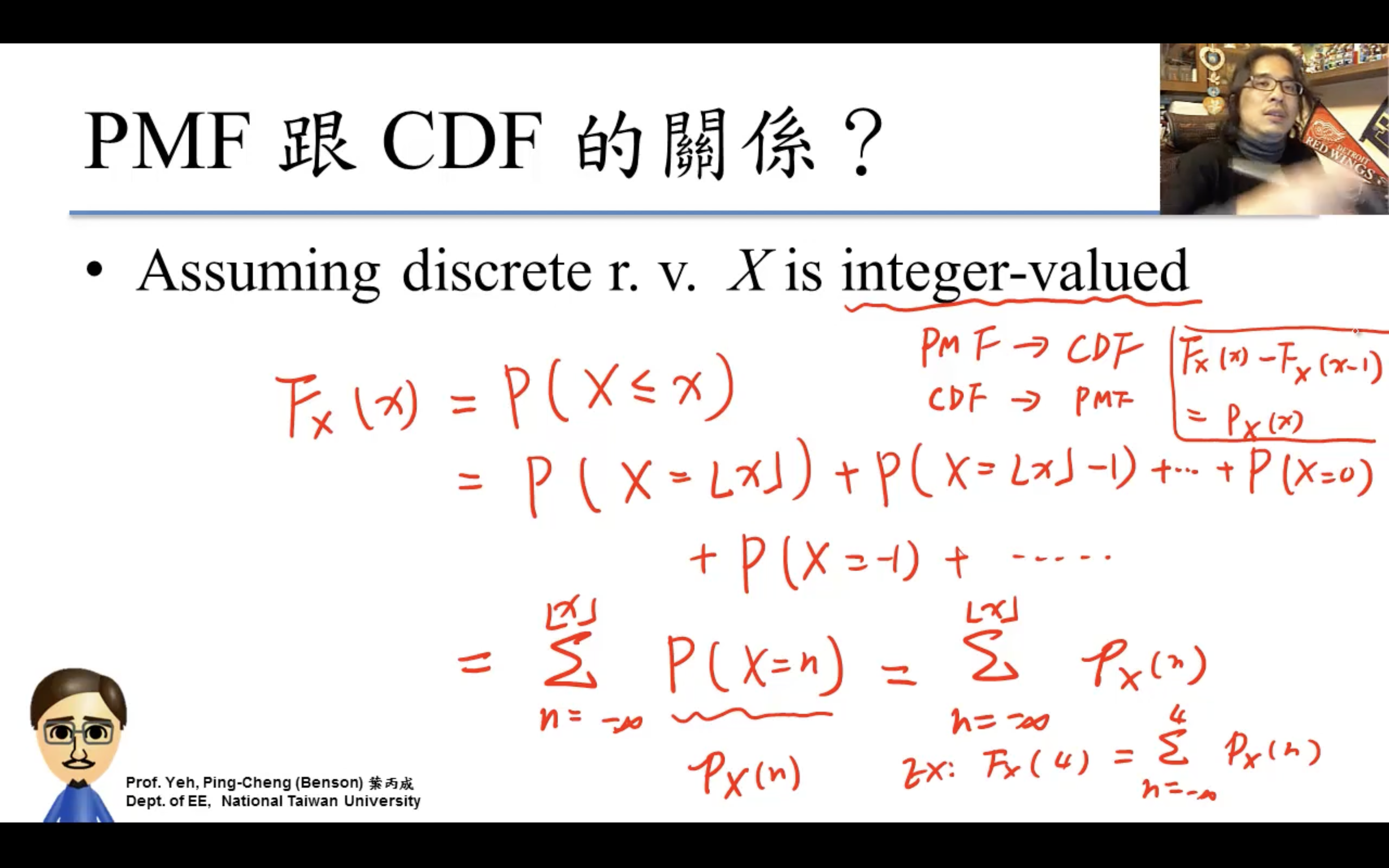
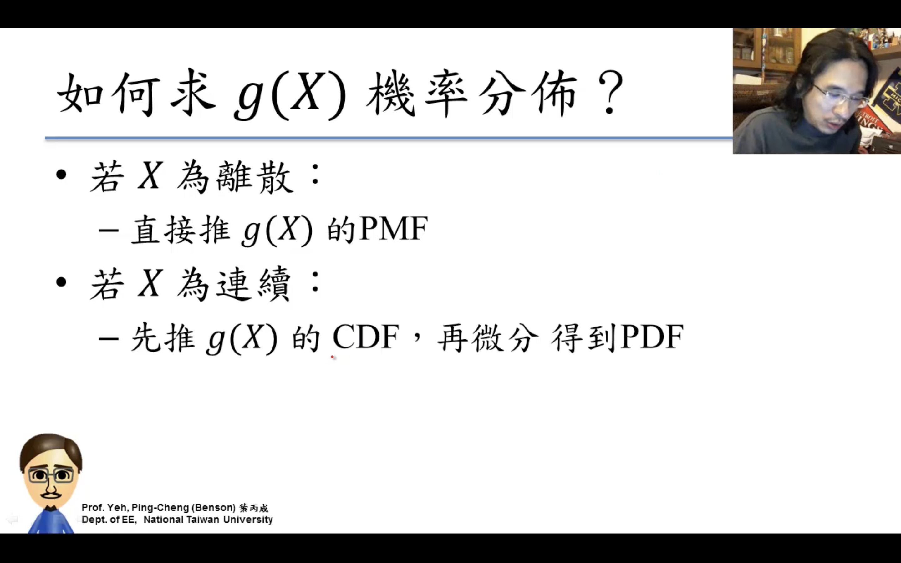
兩個函數一個是X=x(PMF)，一個是X<=x(CDF)就是這個區別。
分布是把很多相似實驗總結成規律。

Discrete Probability Distributions

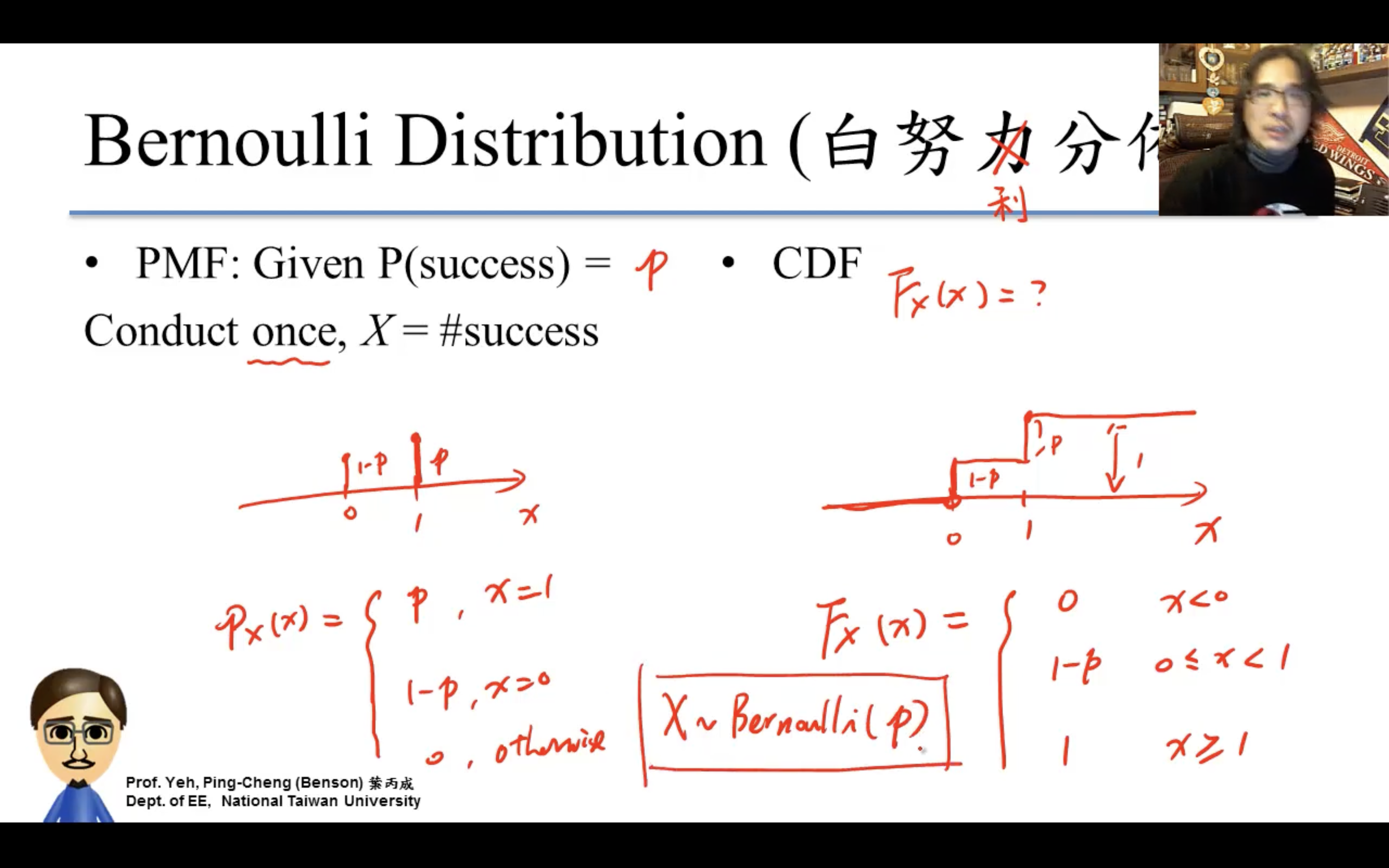
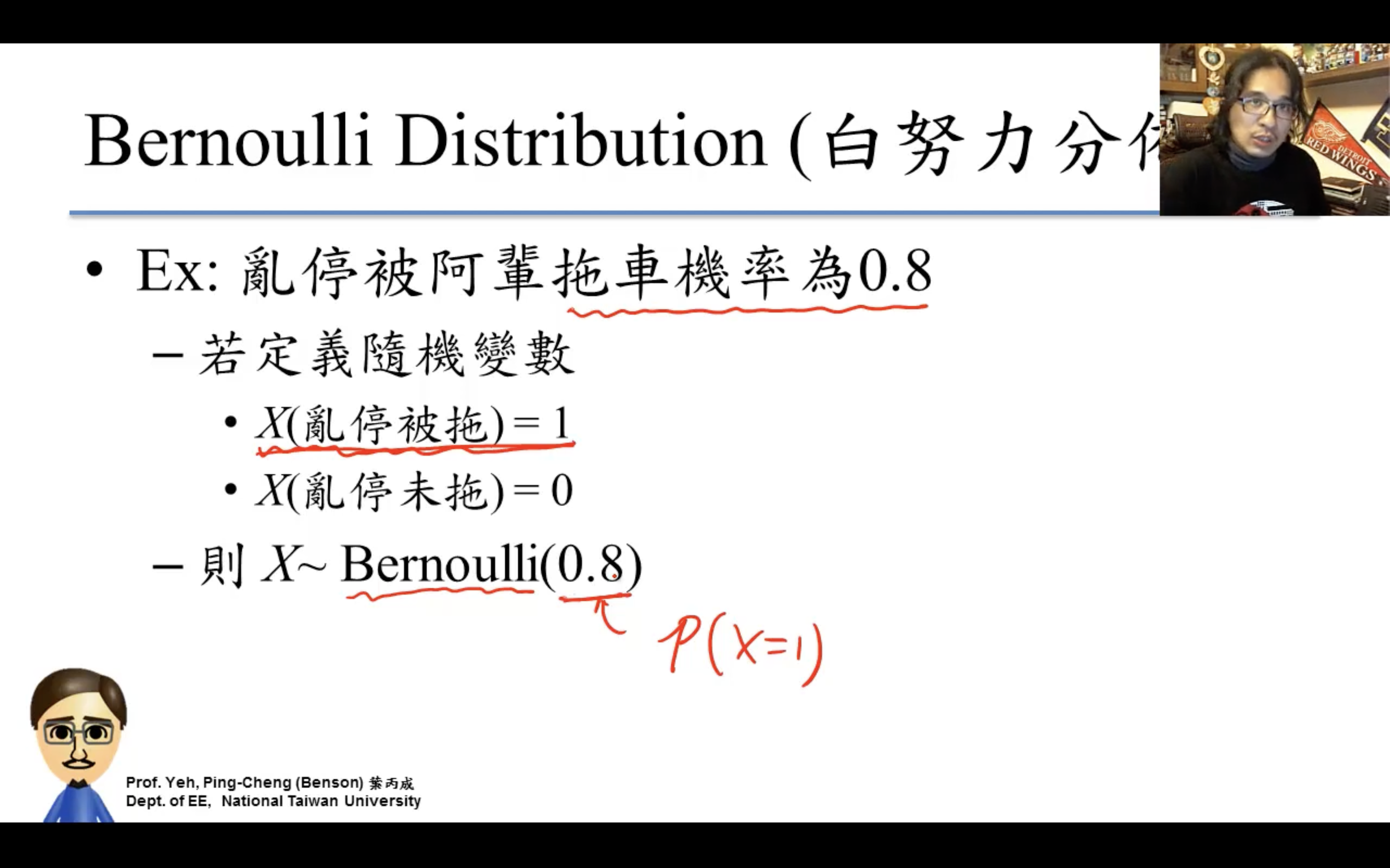
Bernoulli Distribution

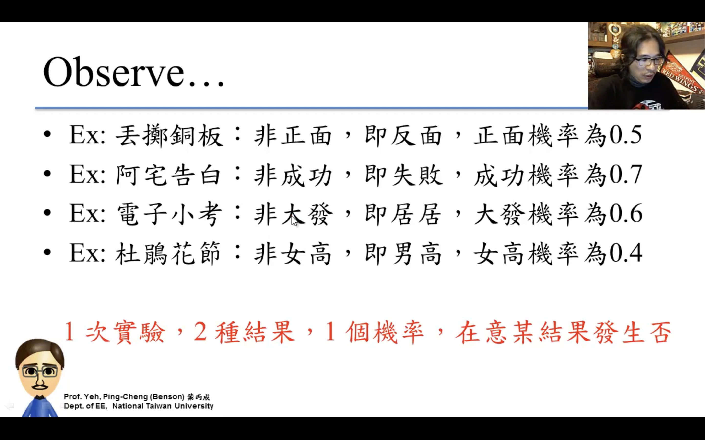
只care成功失敗，一次實驗，非1即0。

Binomial Distribution

二項分布。

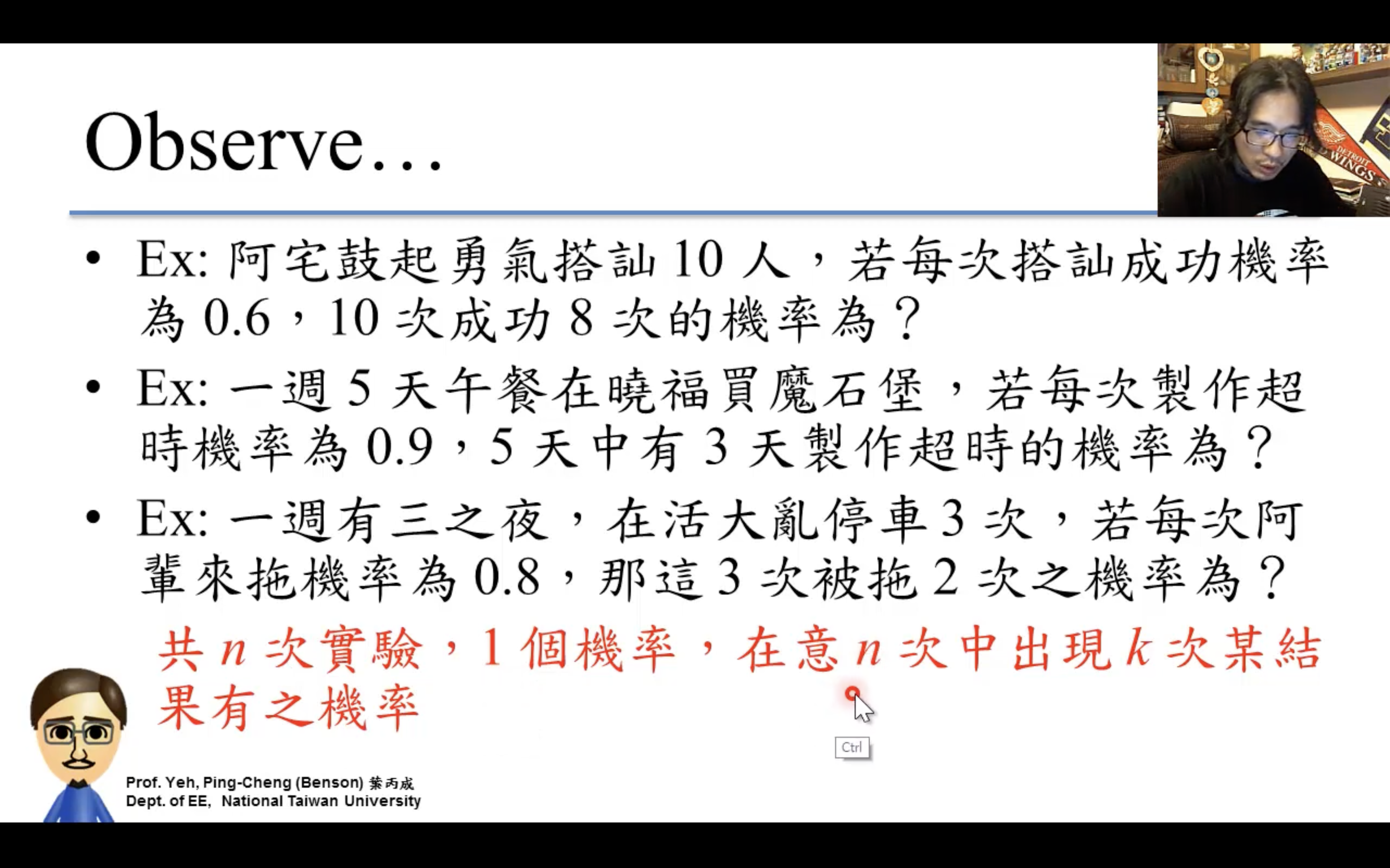
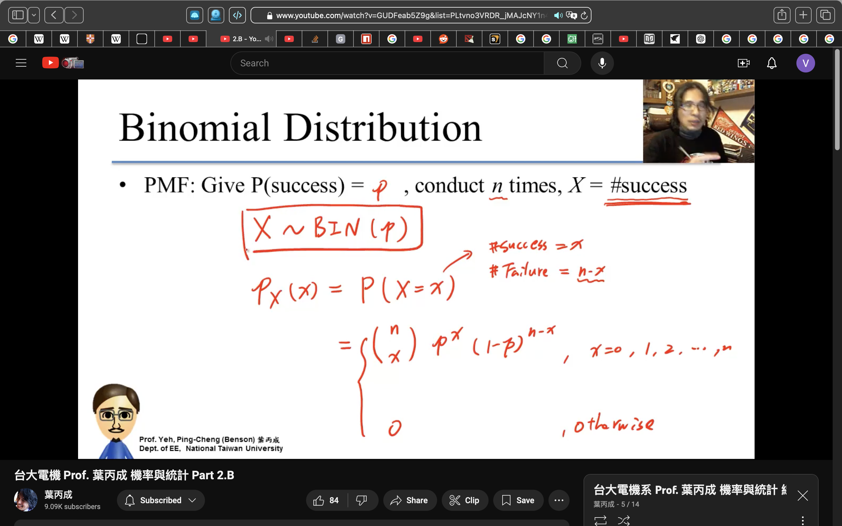
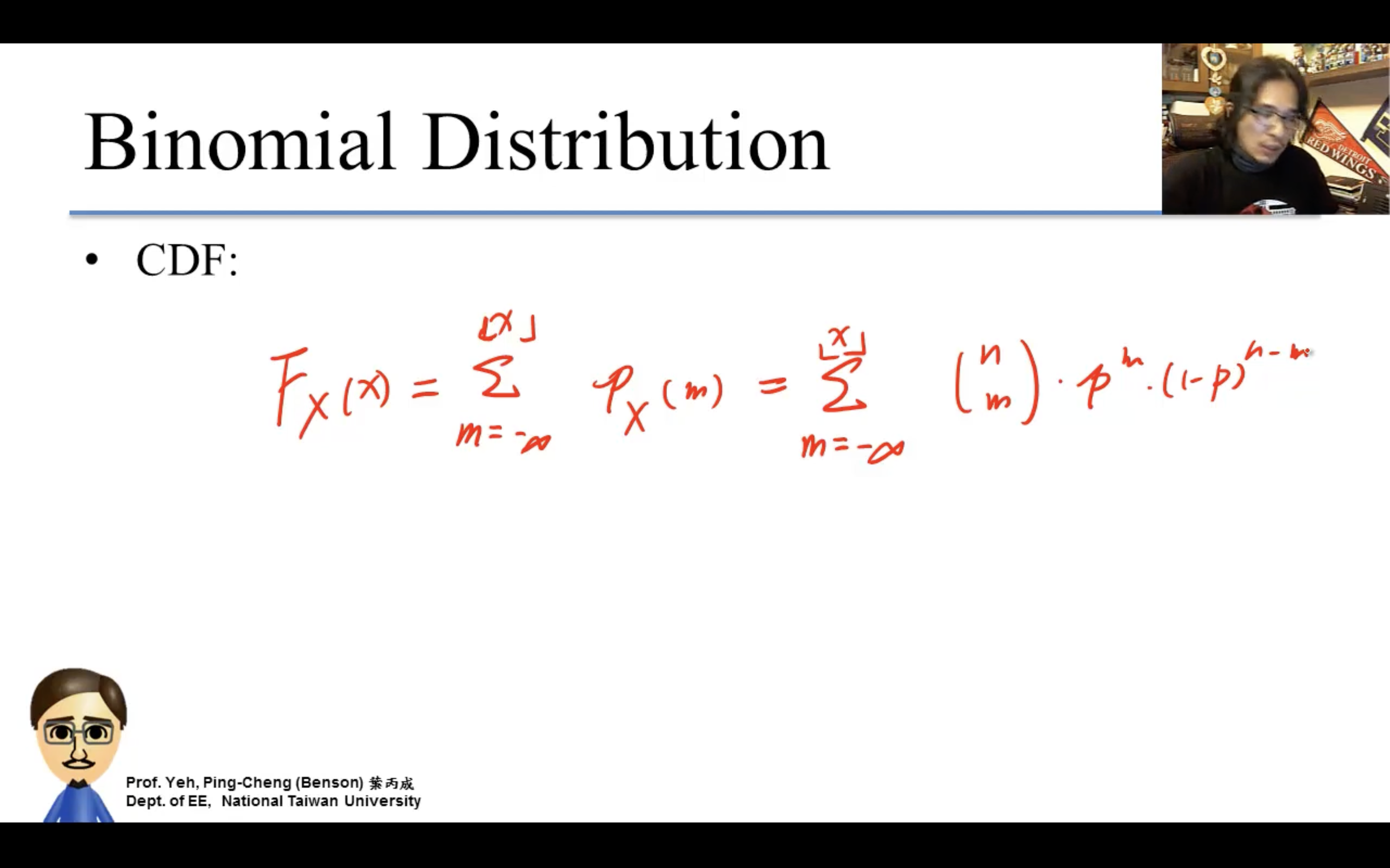
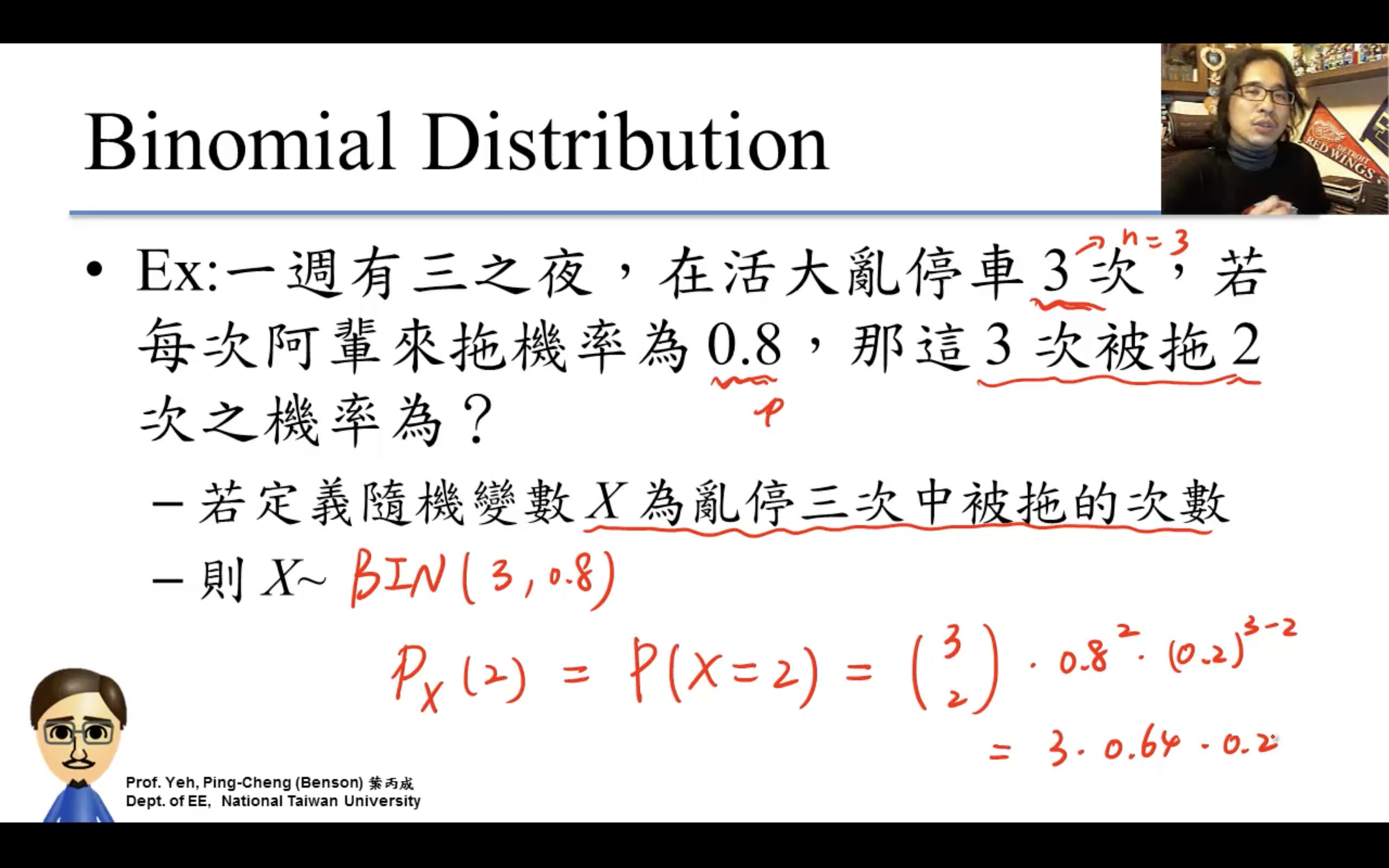
n=1時退化成白努力分布。

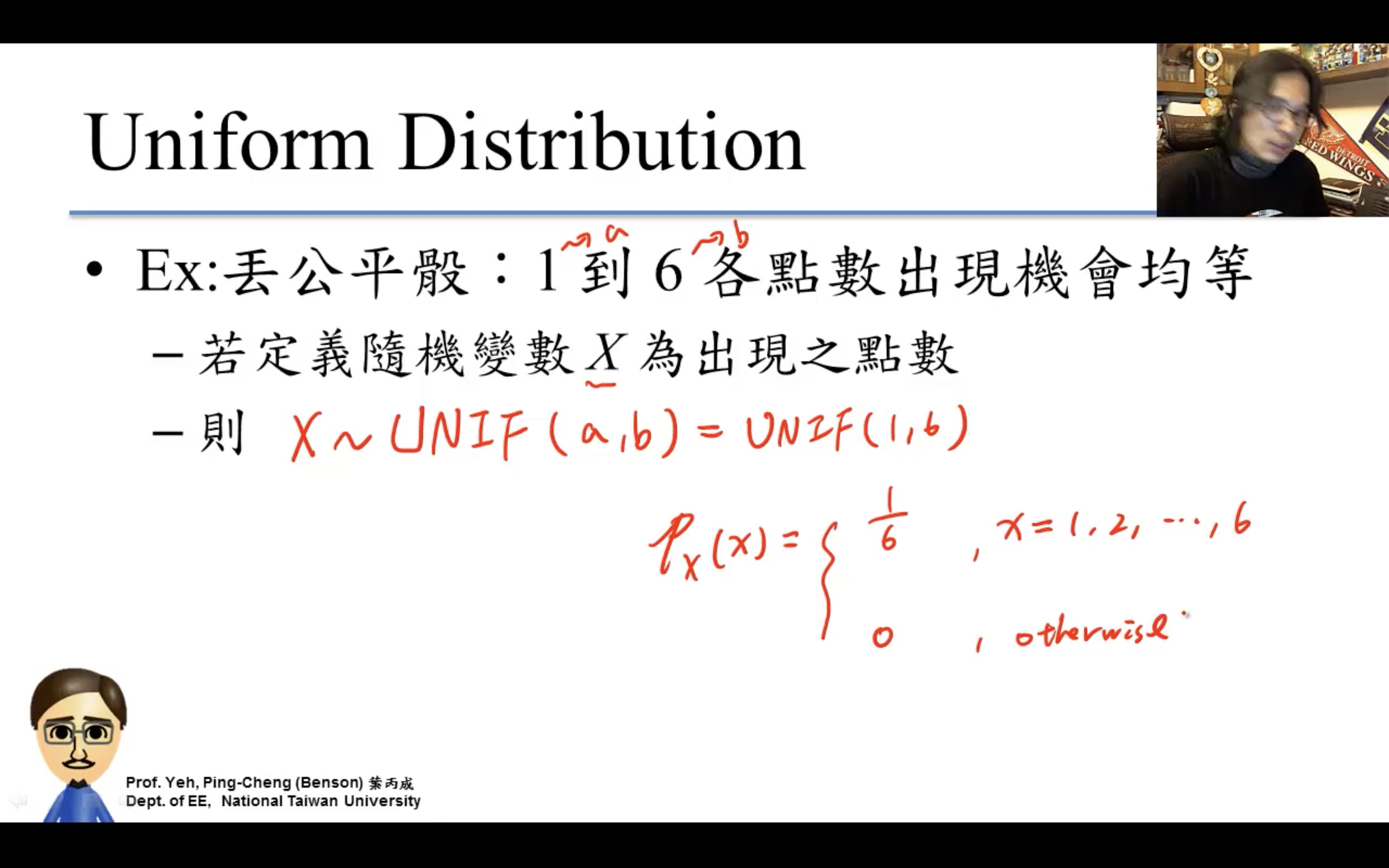
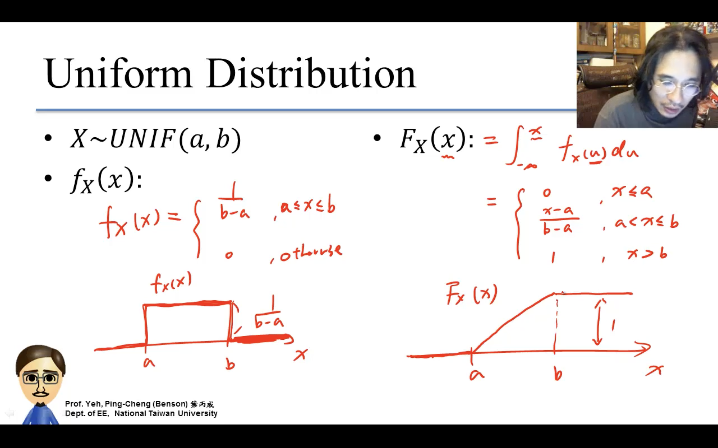
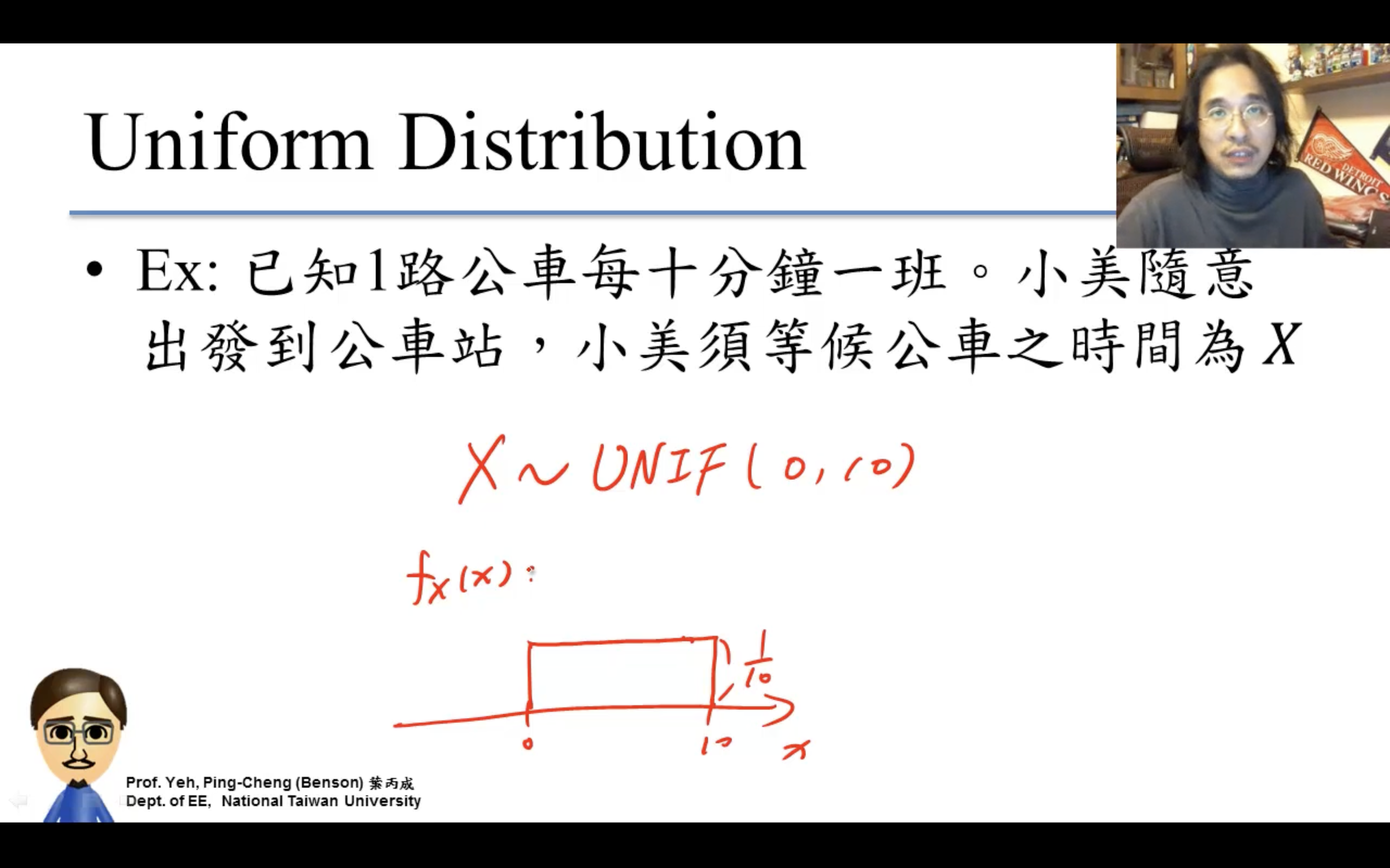
Uniform Distribution

均勻分布。

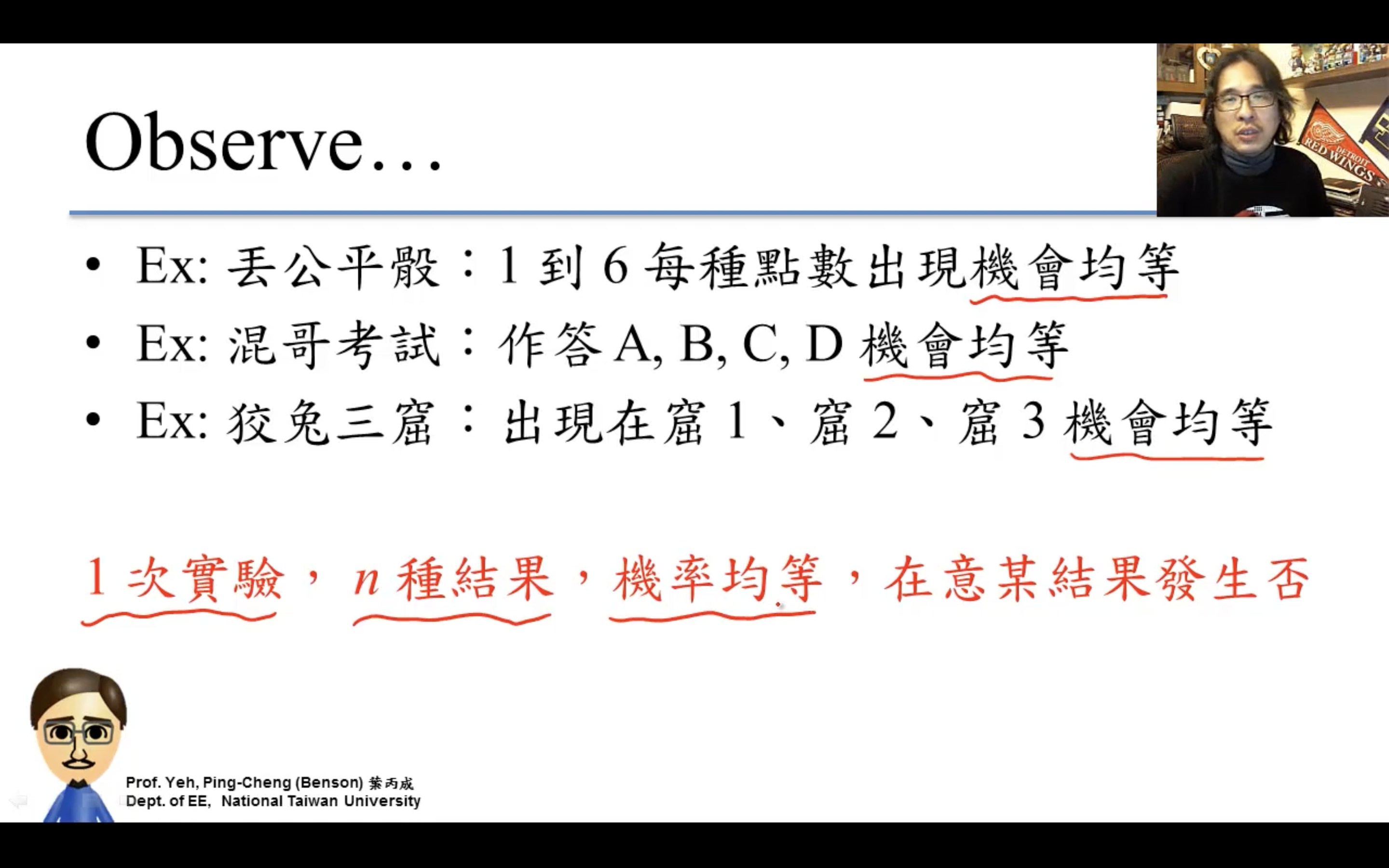
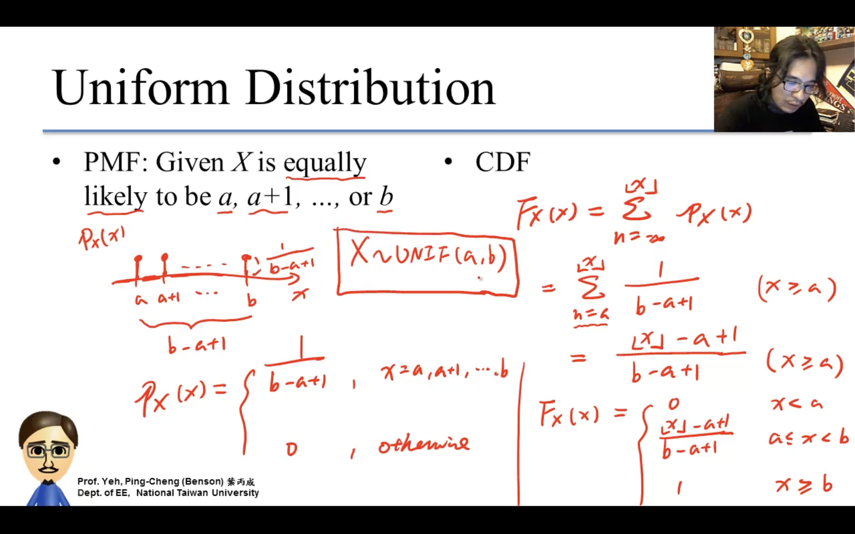
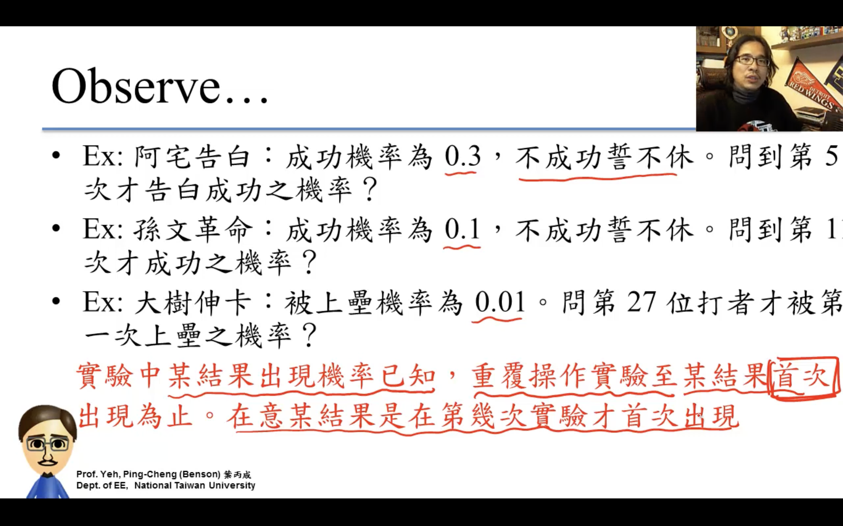
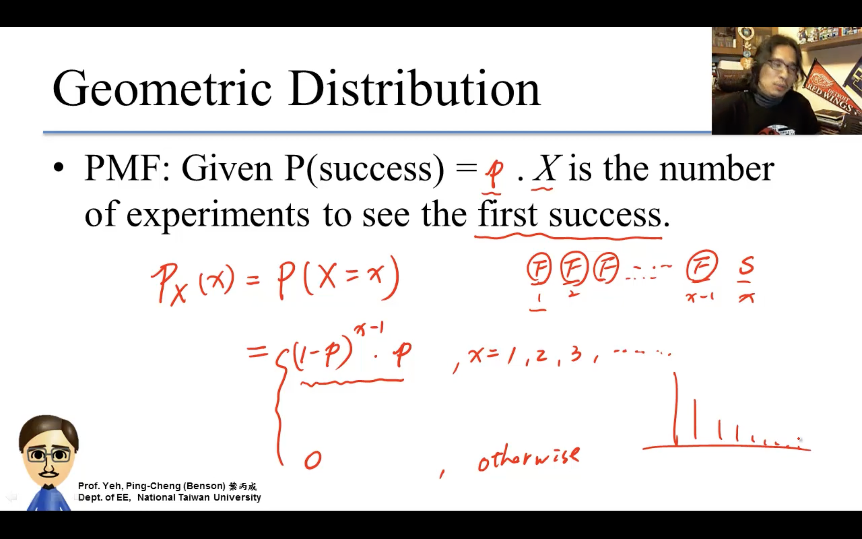
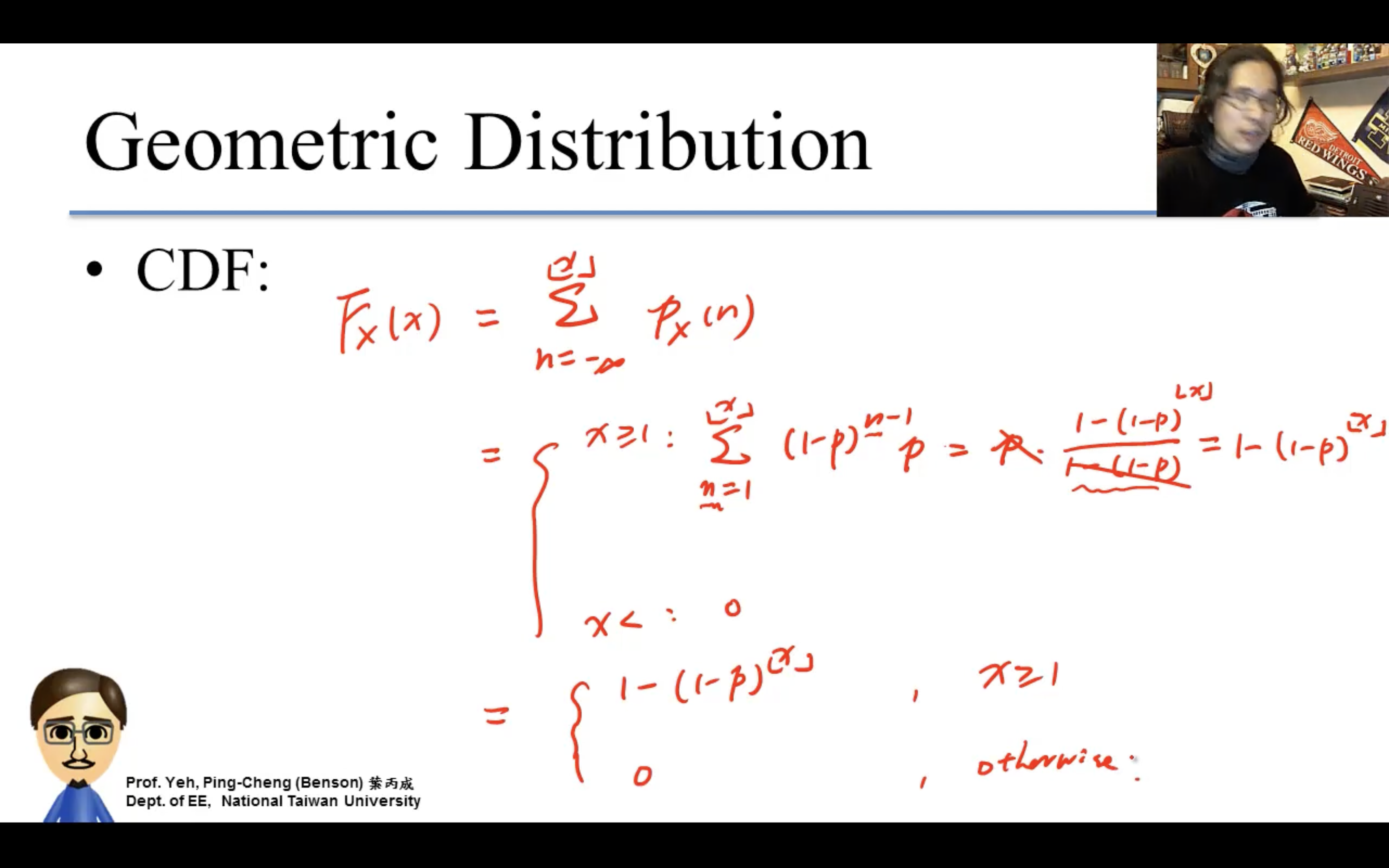
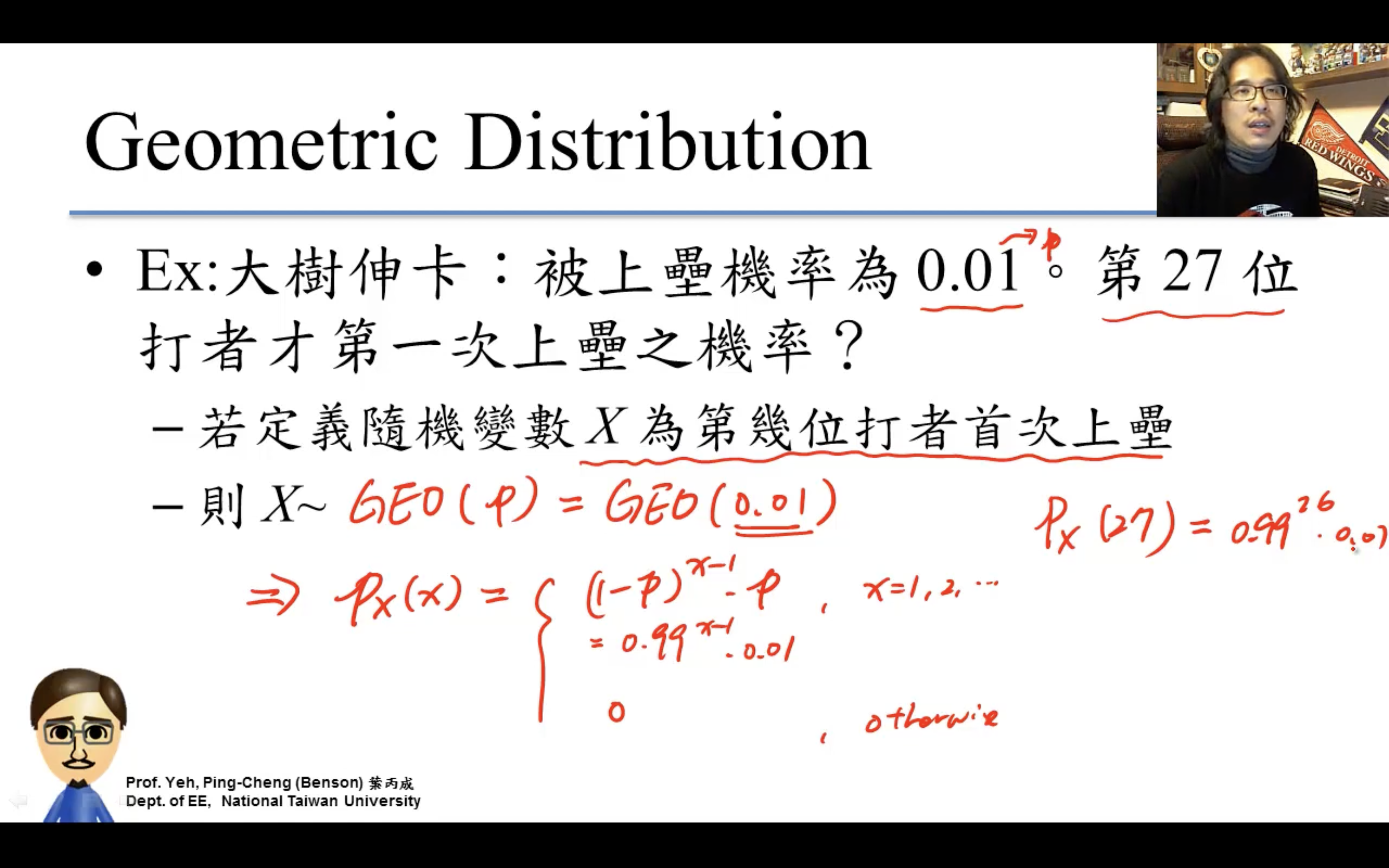
Geometric Distribution

几何分布。

$P_X(x)$等比級數，即幾何級數

$S_n=\frac{a_1\left(1-r^n\right)}{1-r}, r \neq 1$

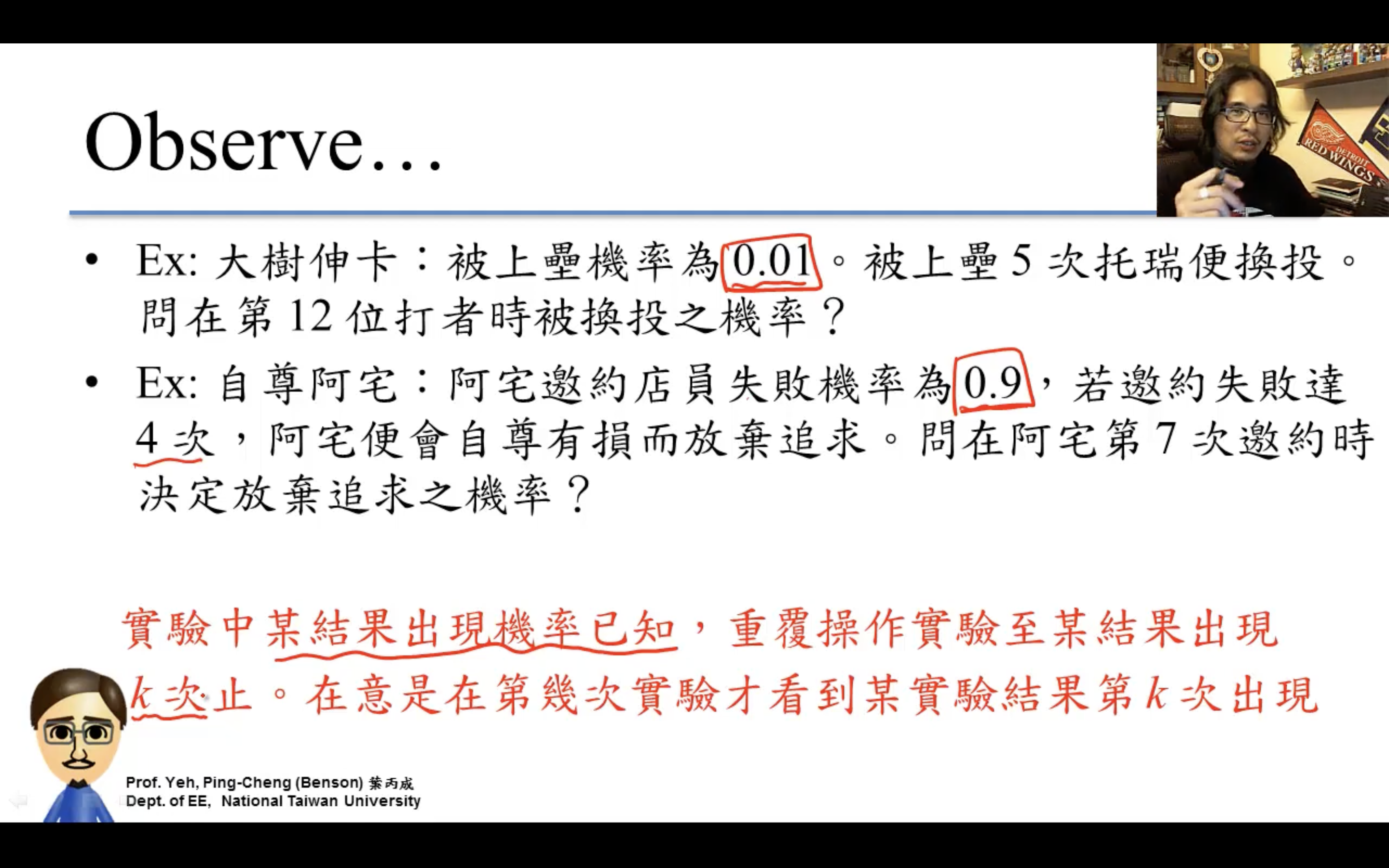
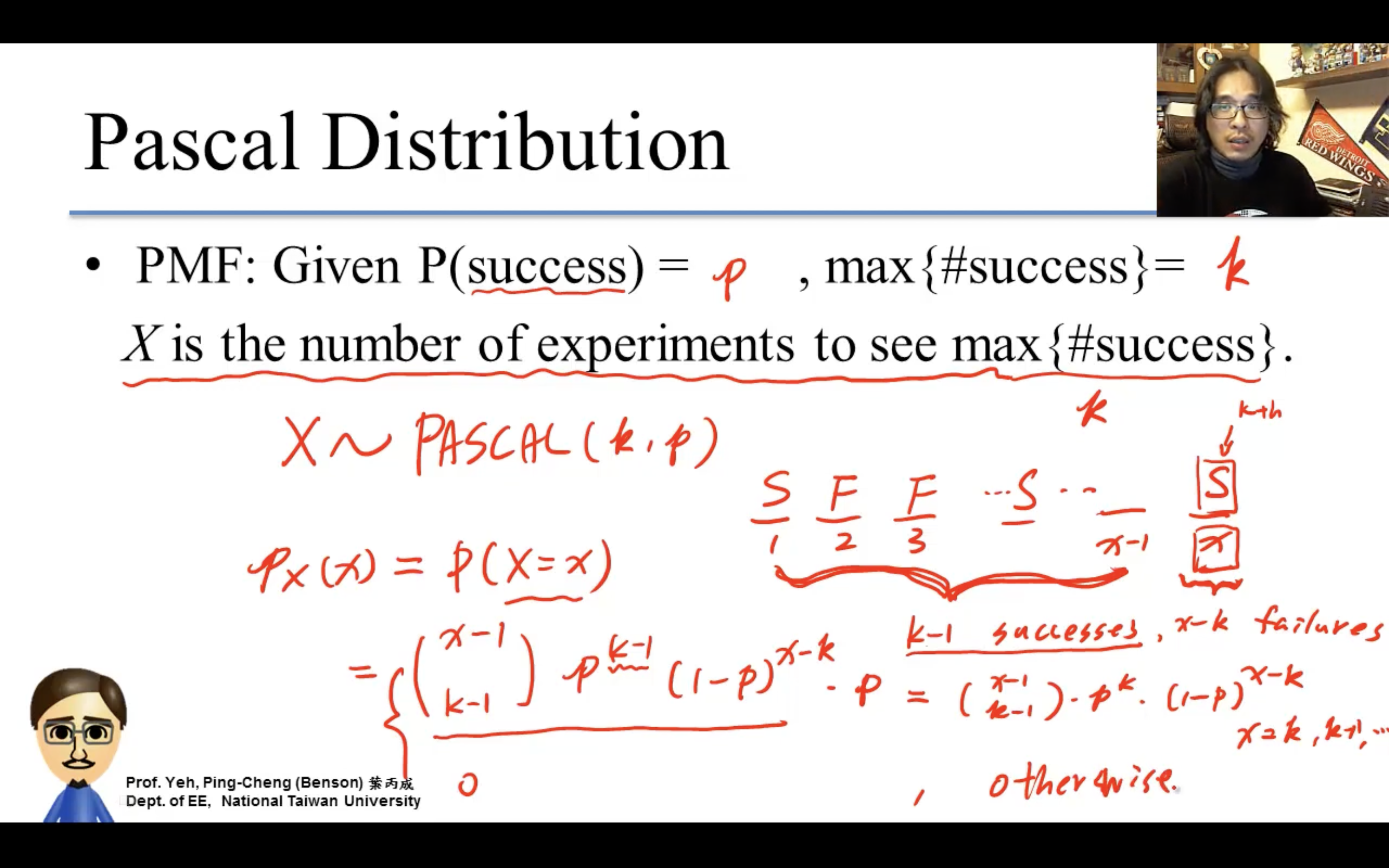
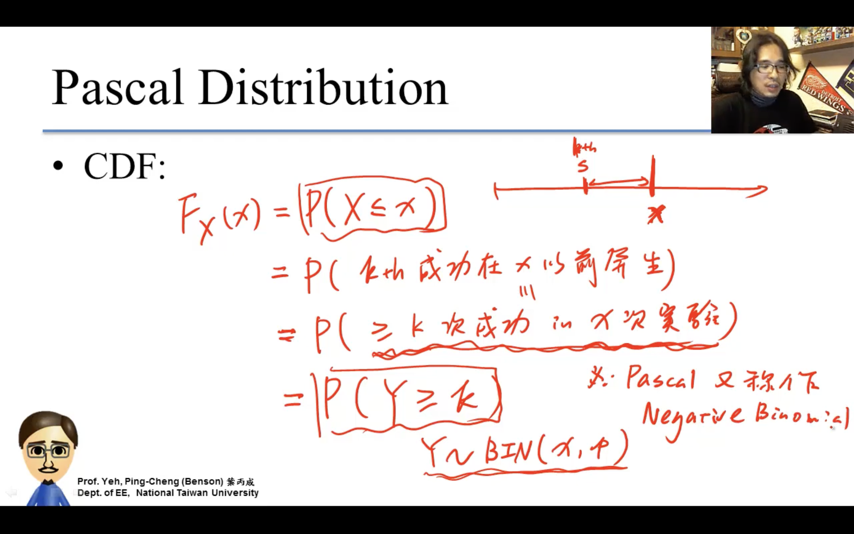
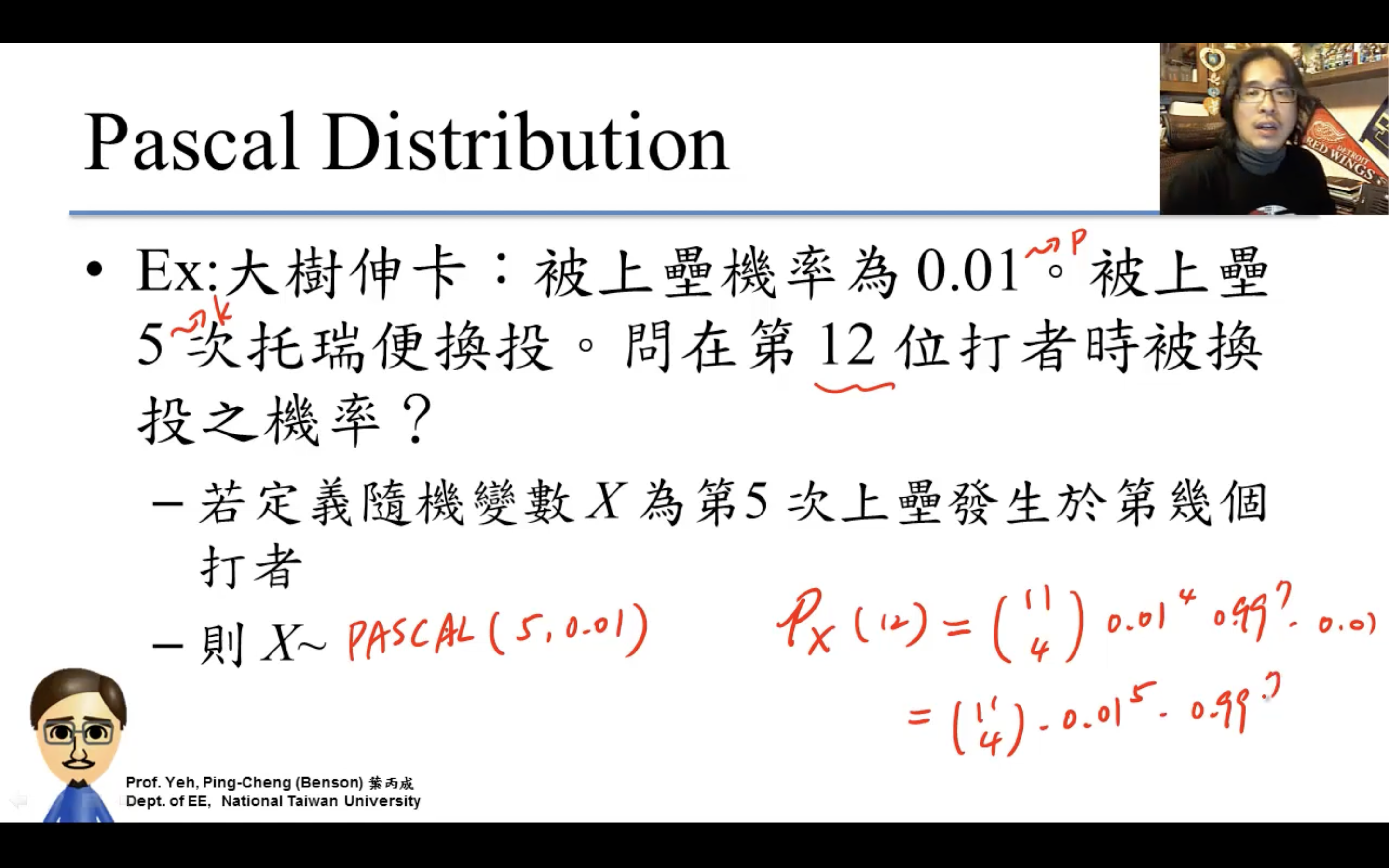
Pascal Distribution

k=1就退化成Geometric分布。

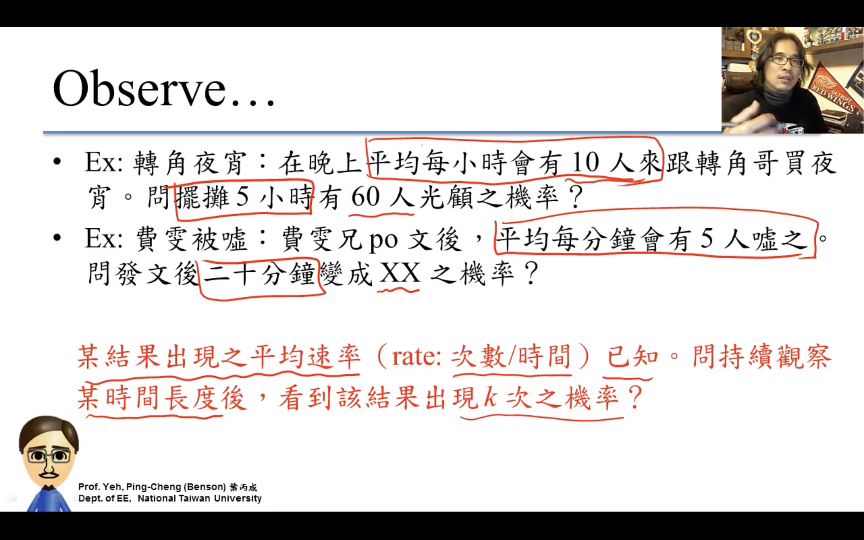
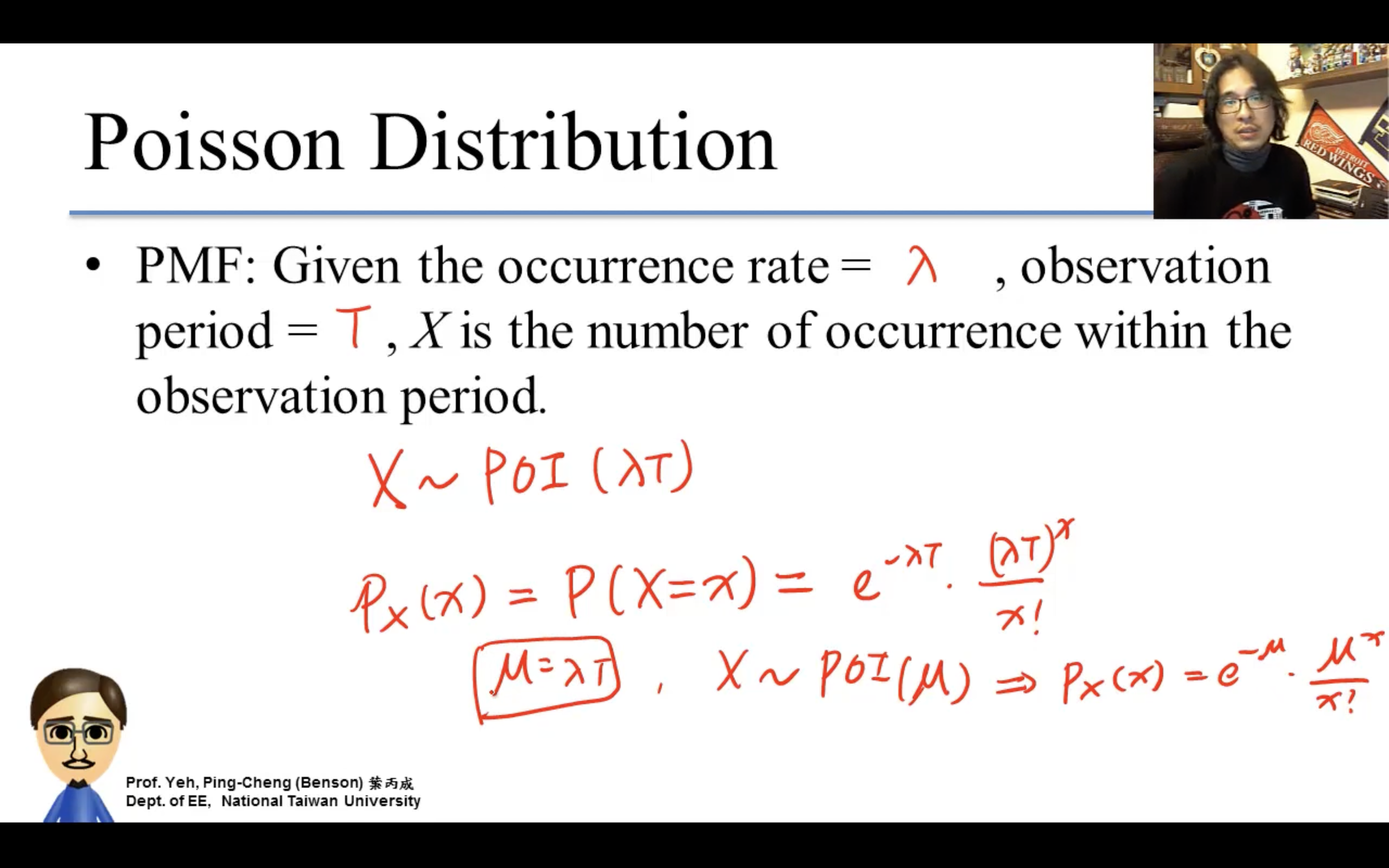
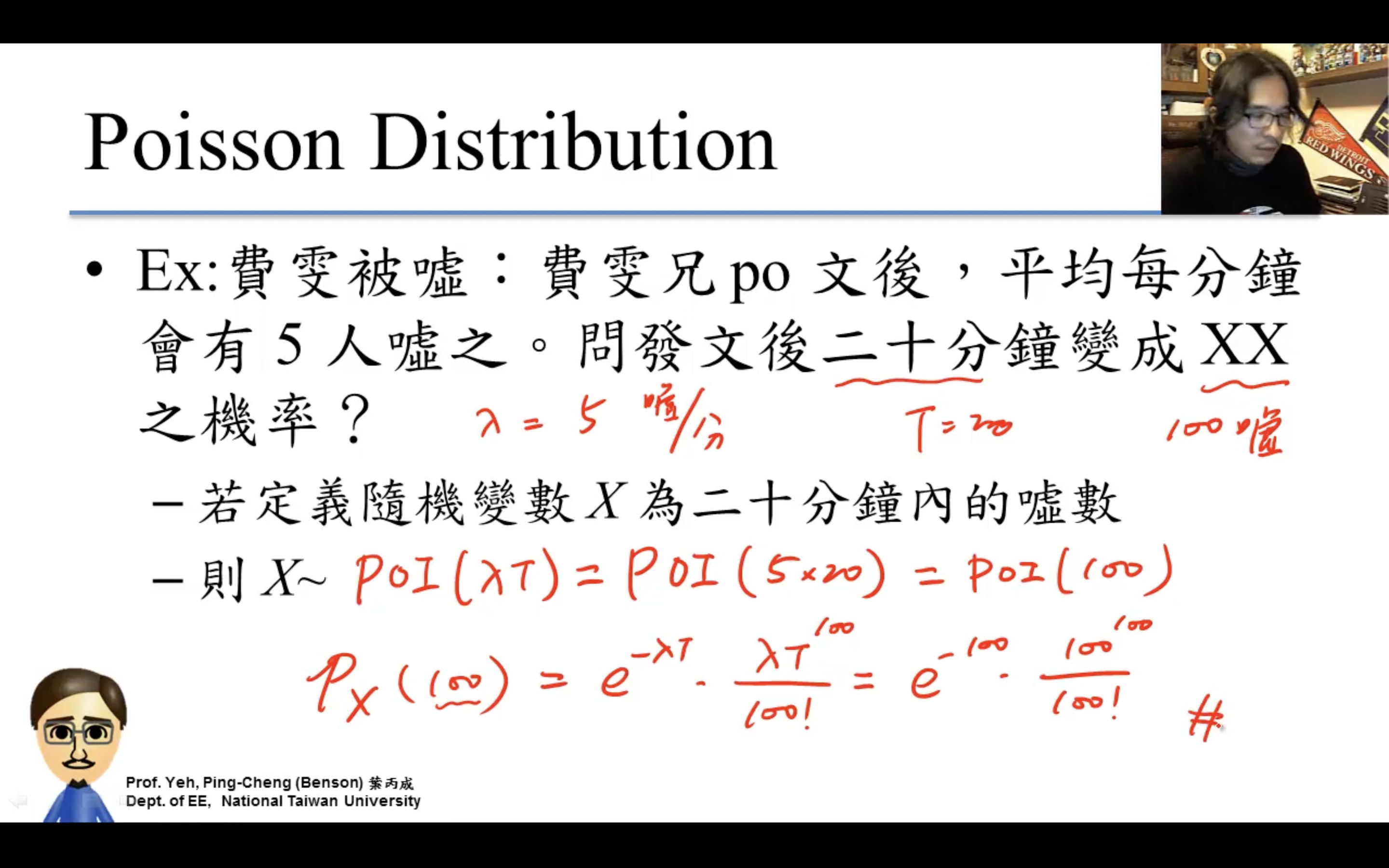
Poisson Distribution

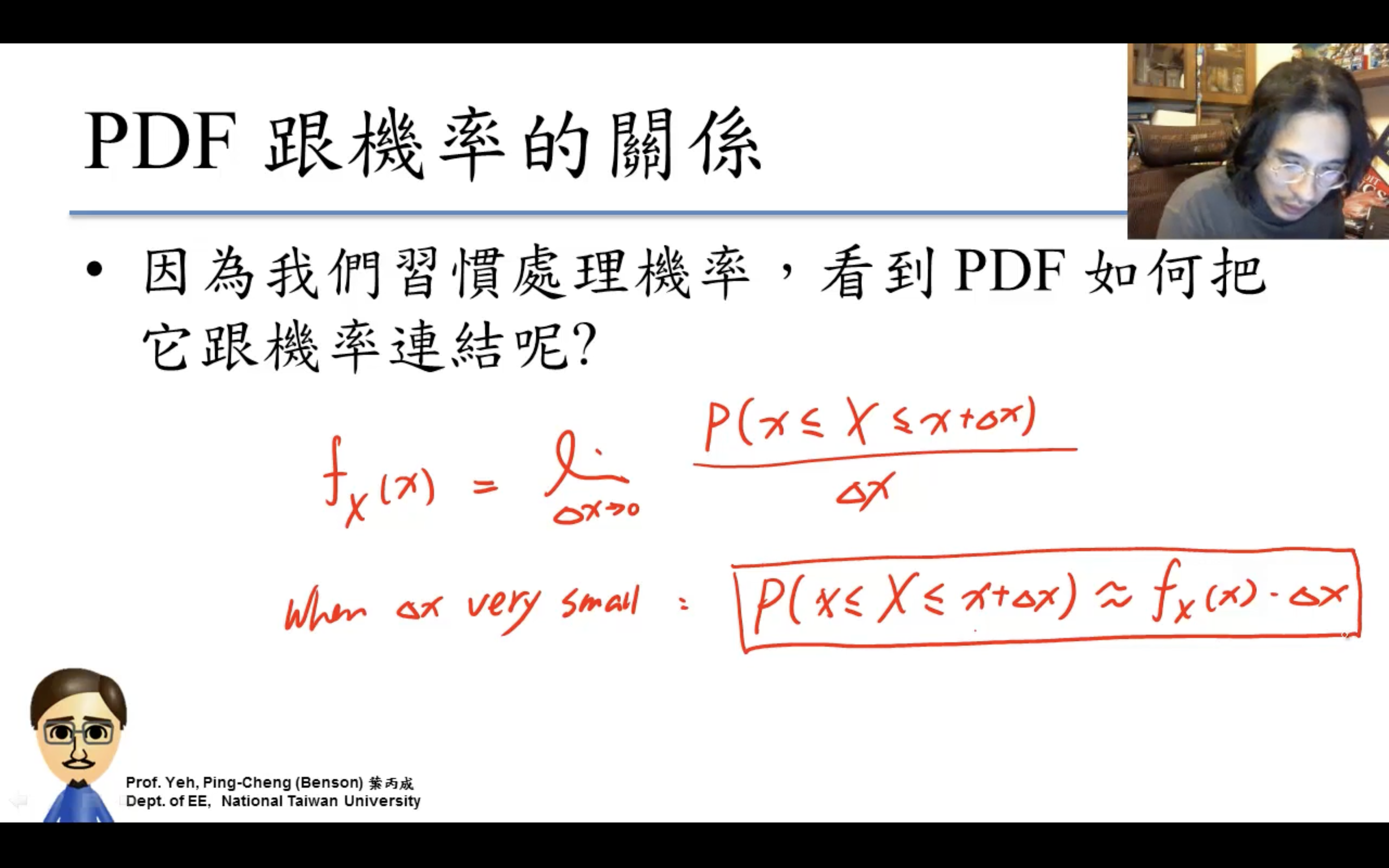
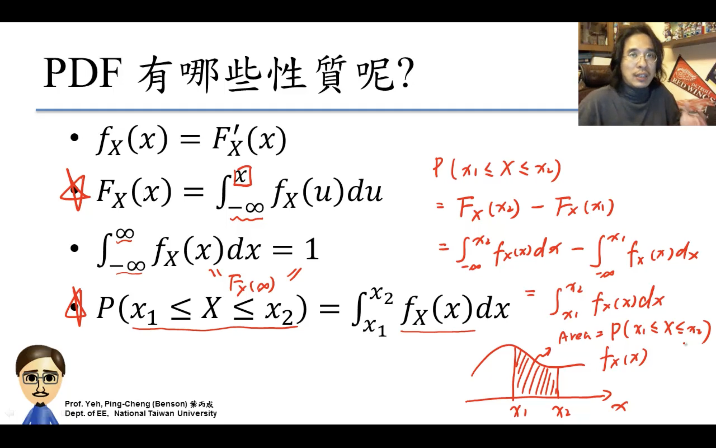
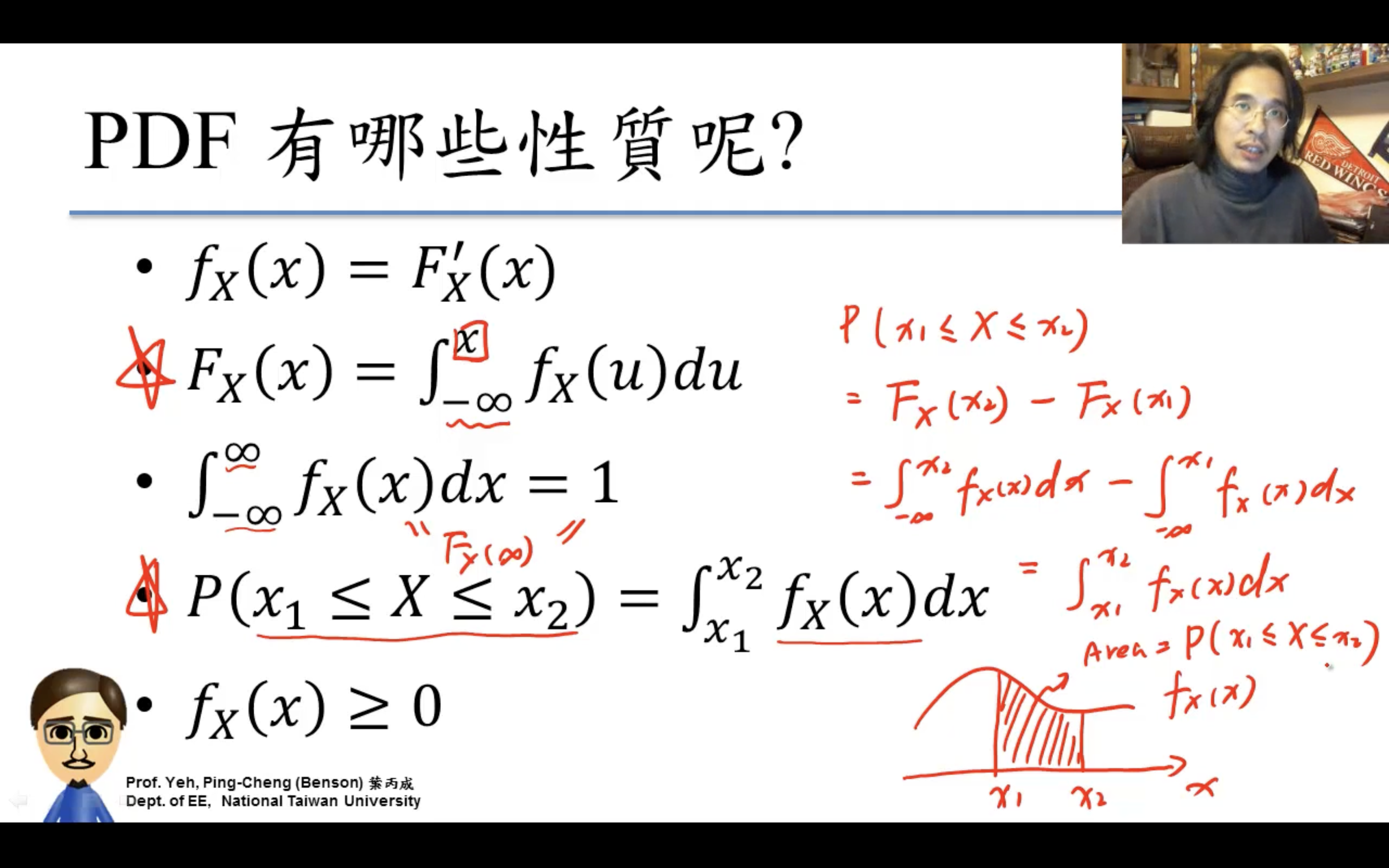
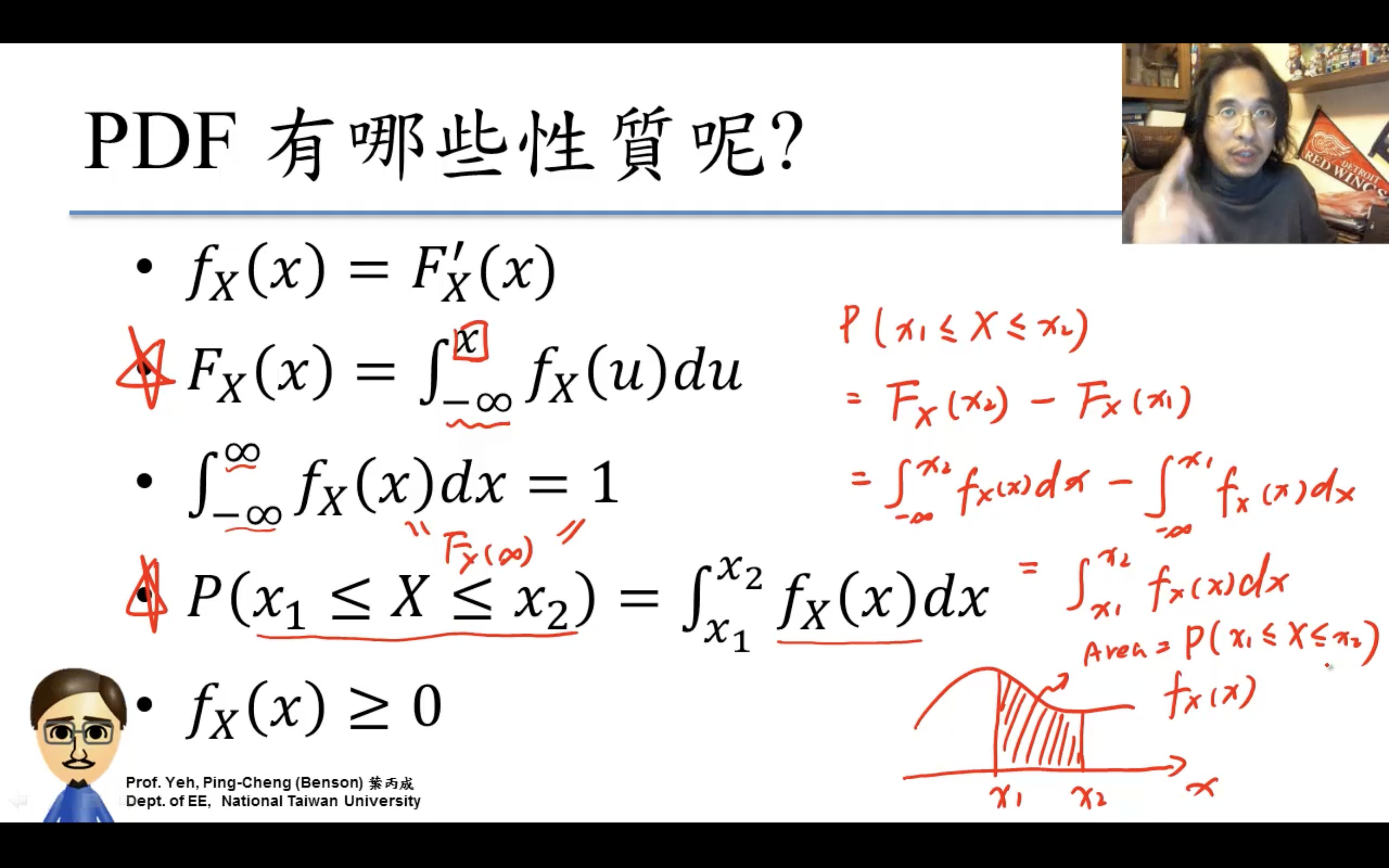
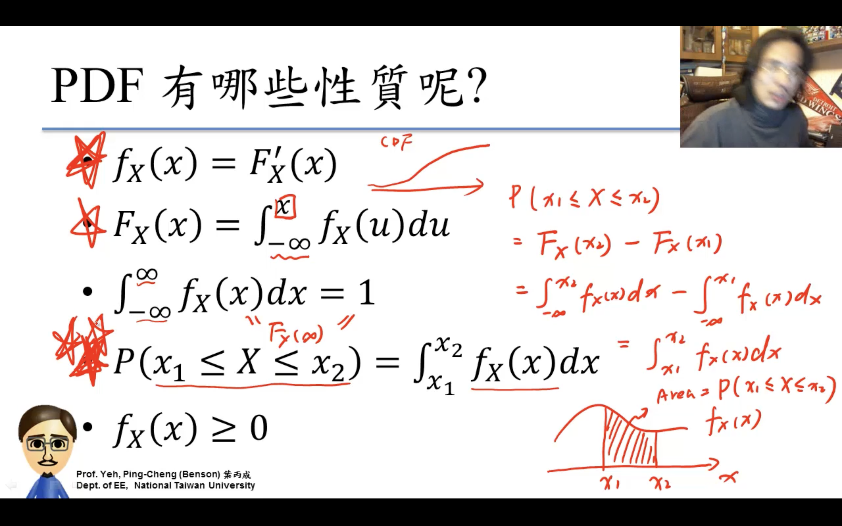
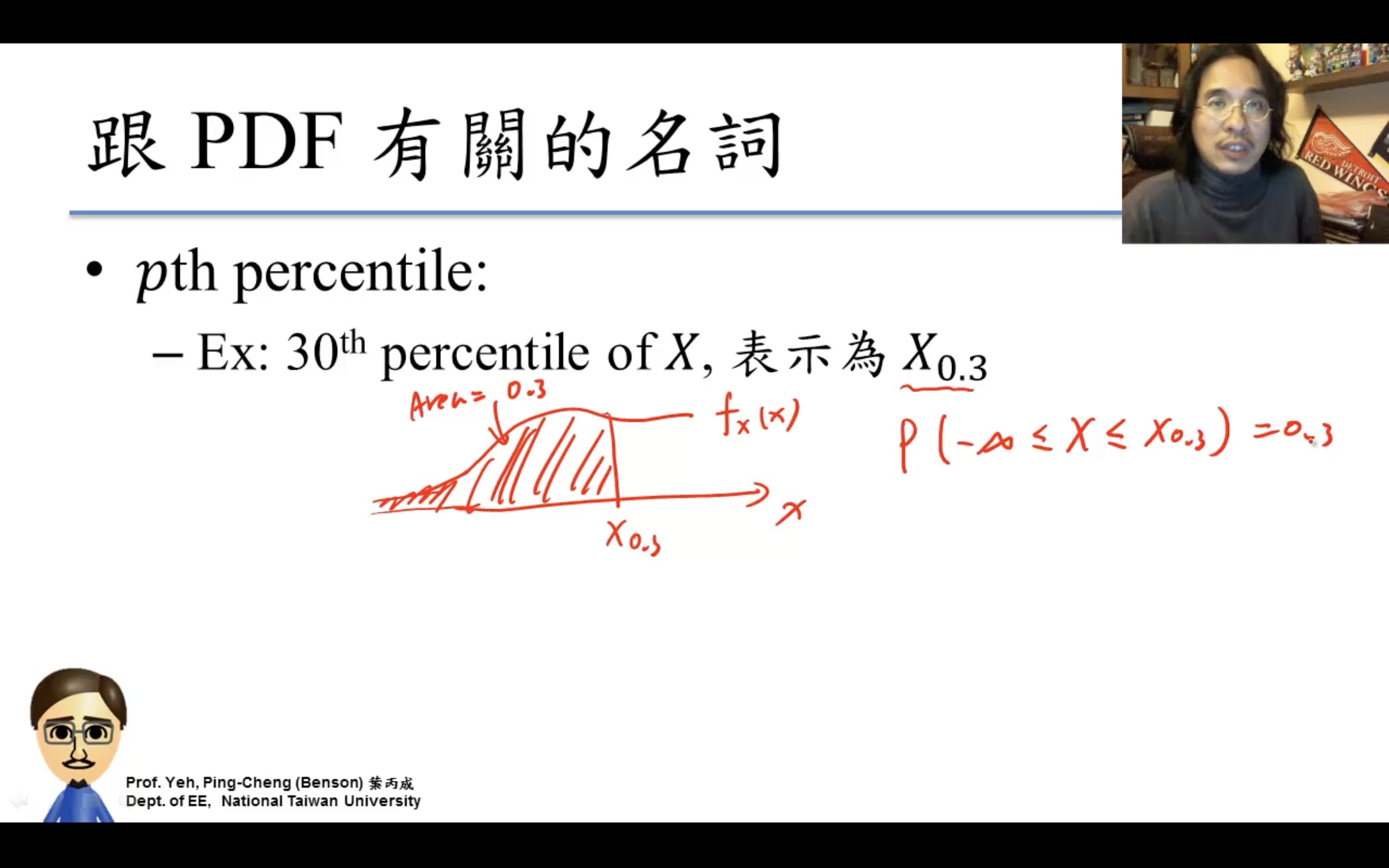
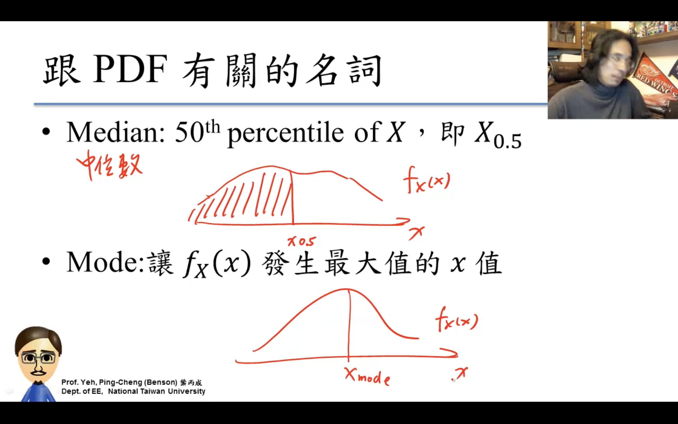
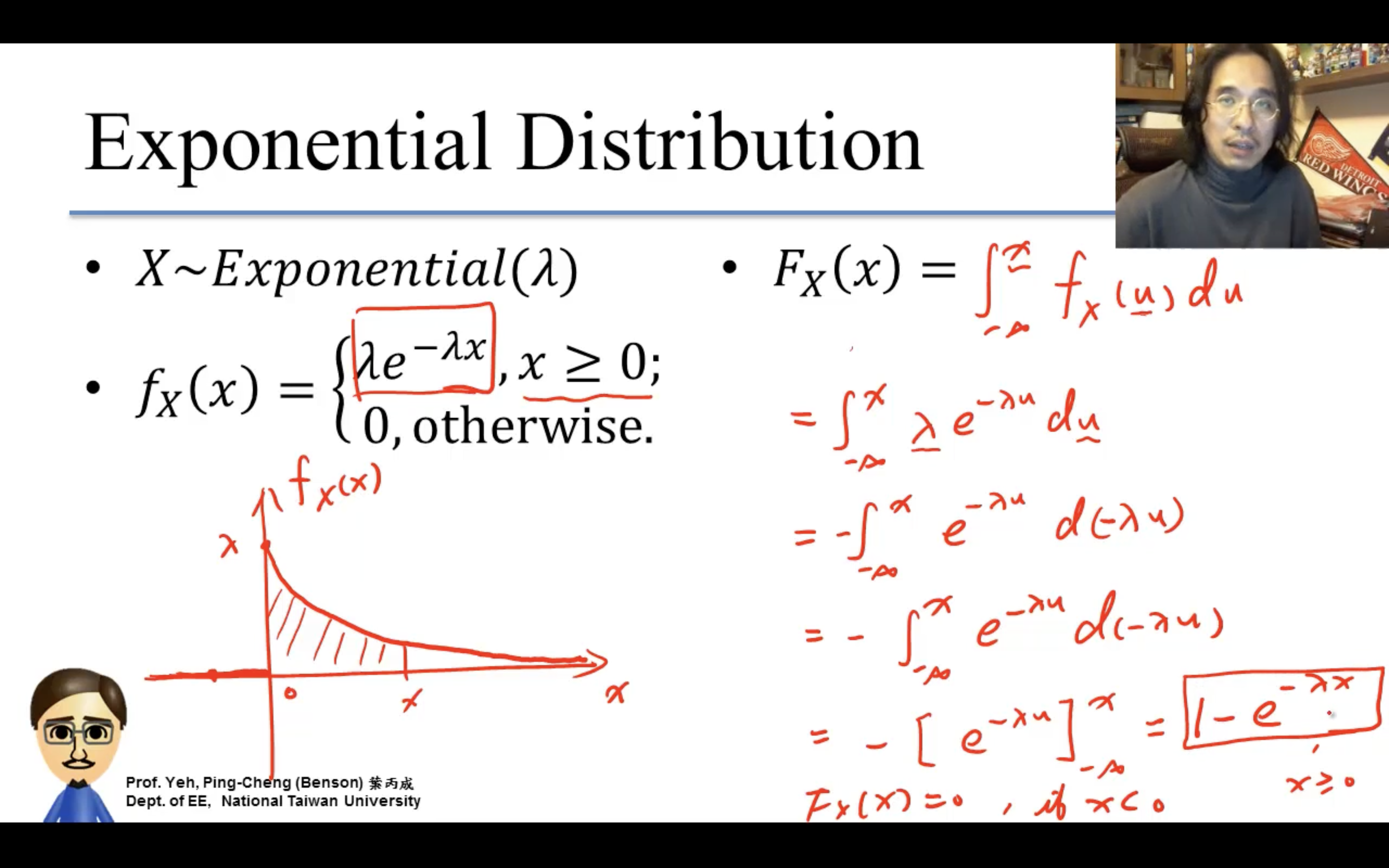
Probability Density Function

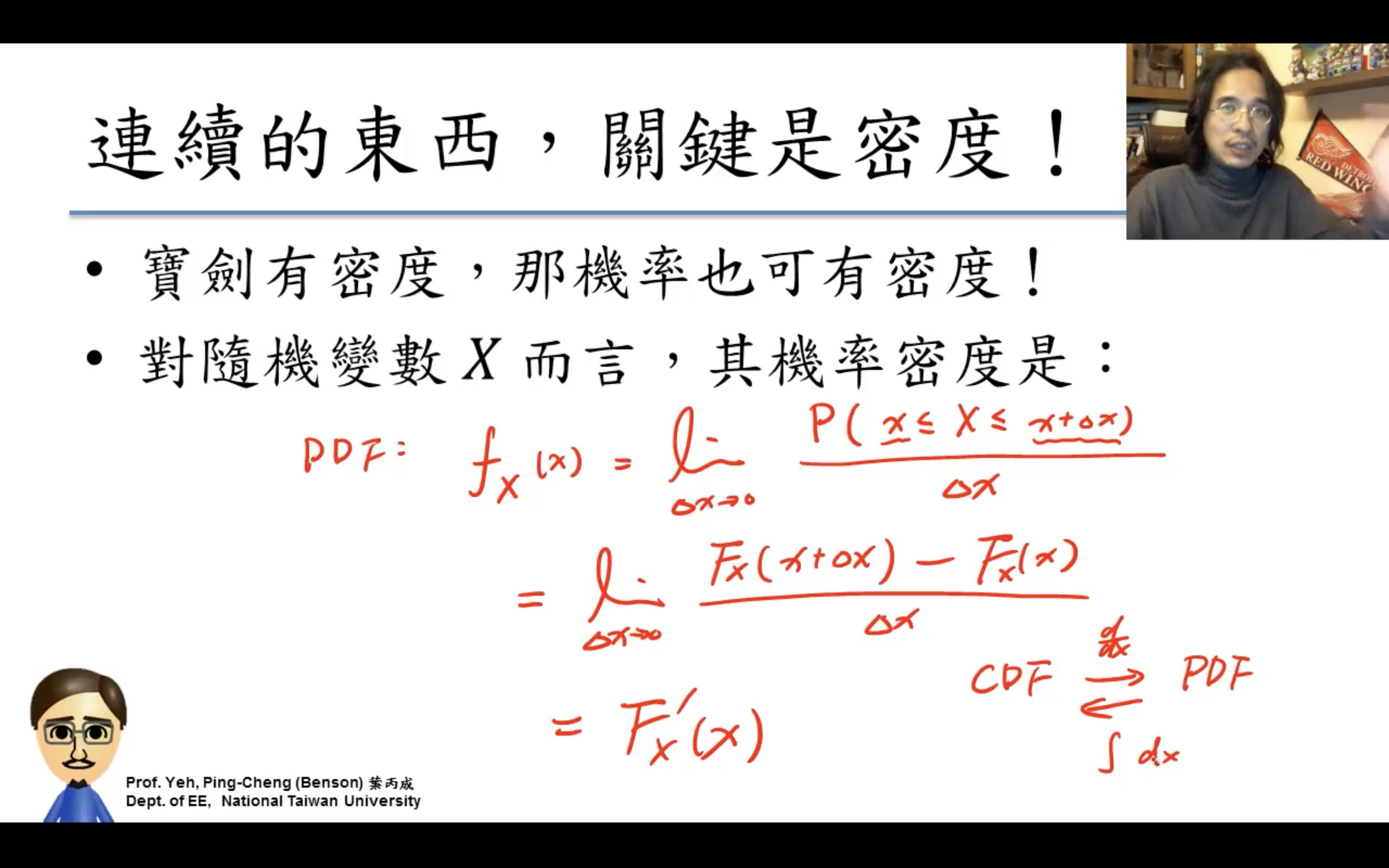
PDF就是CDF的微分！

積分constant不用擔心，可以通過-無窮=0等邊界條件唯一確定。

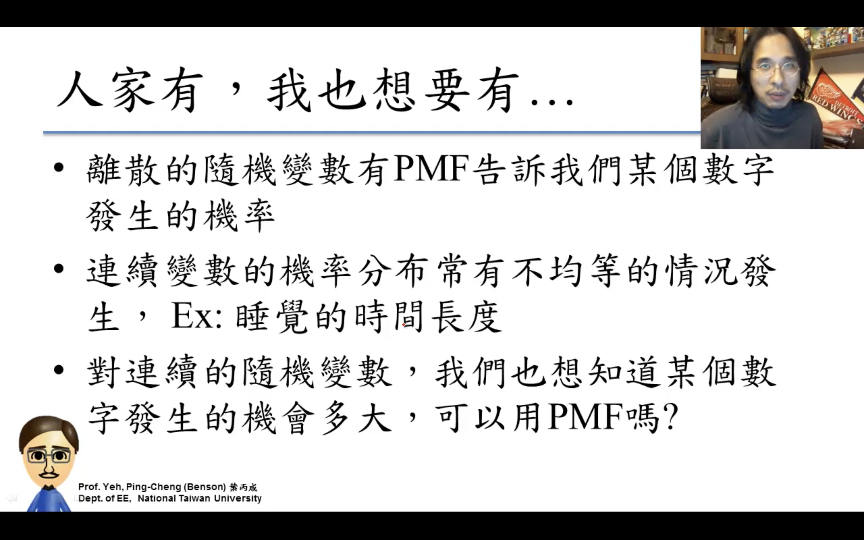
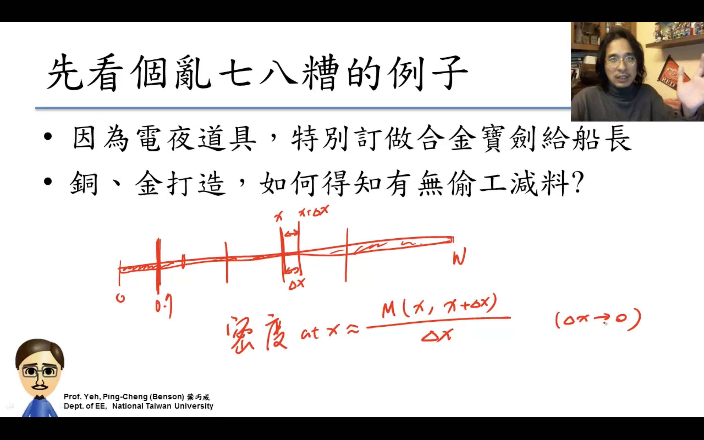
Uniform Distribution

Exponential Distribution

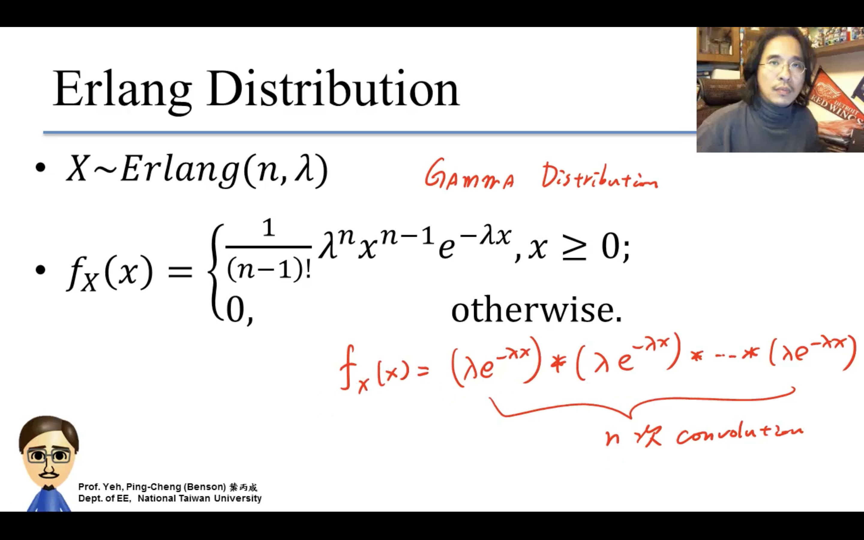
Gamma / Erlang Distribution

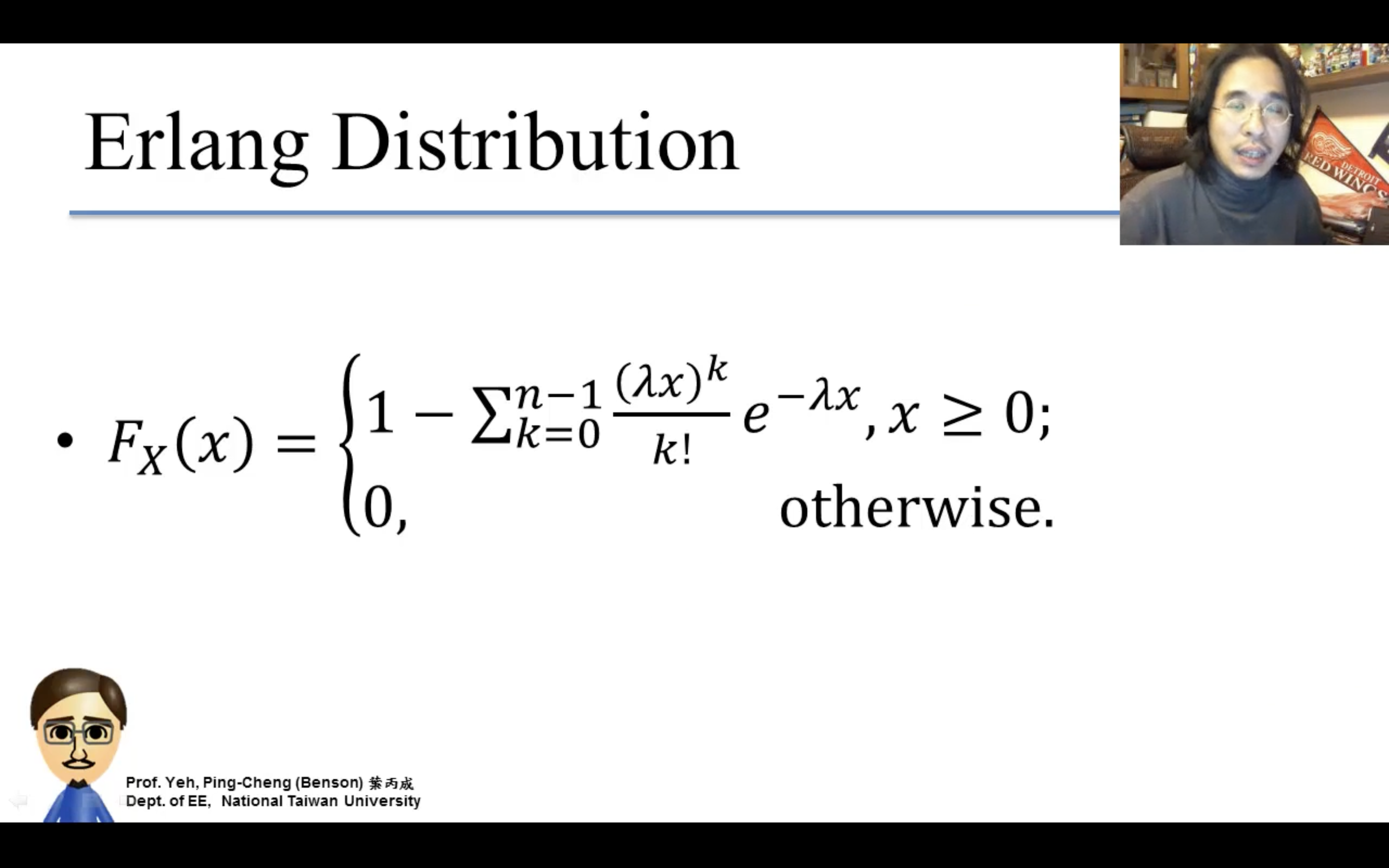
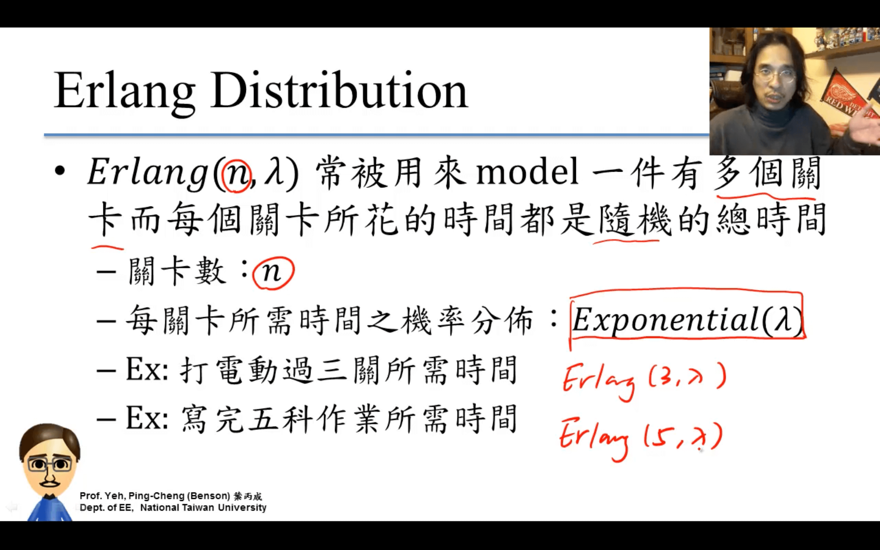
Normal Distribution

終於來到elo的重點。

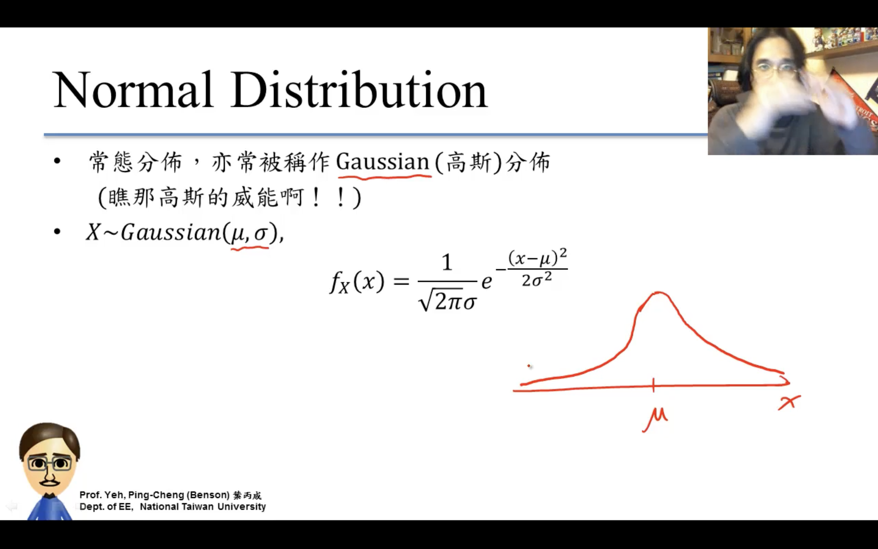
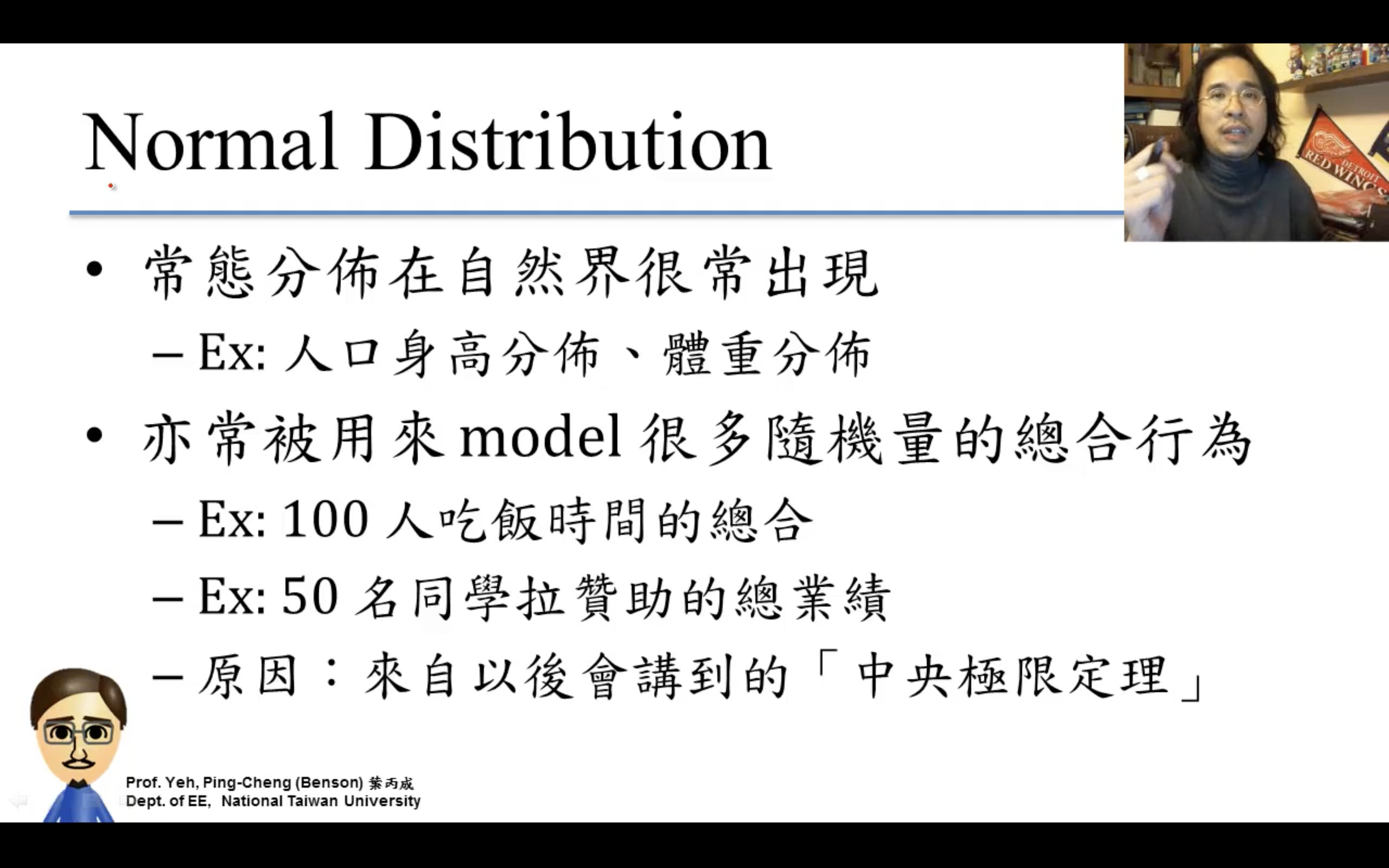
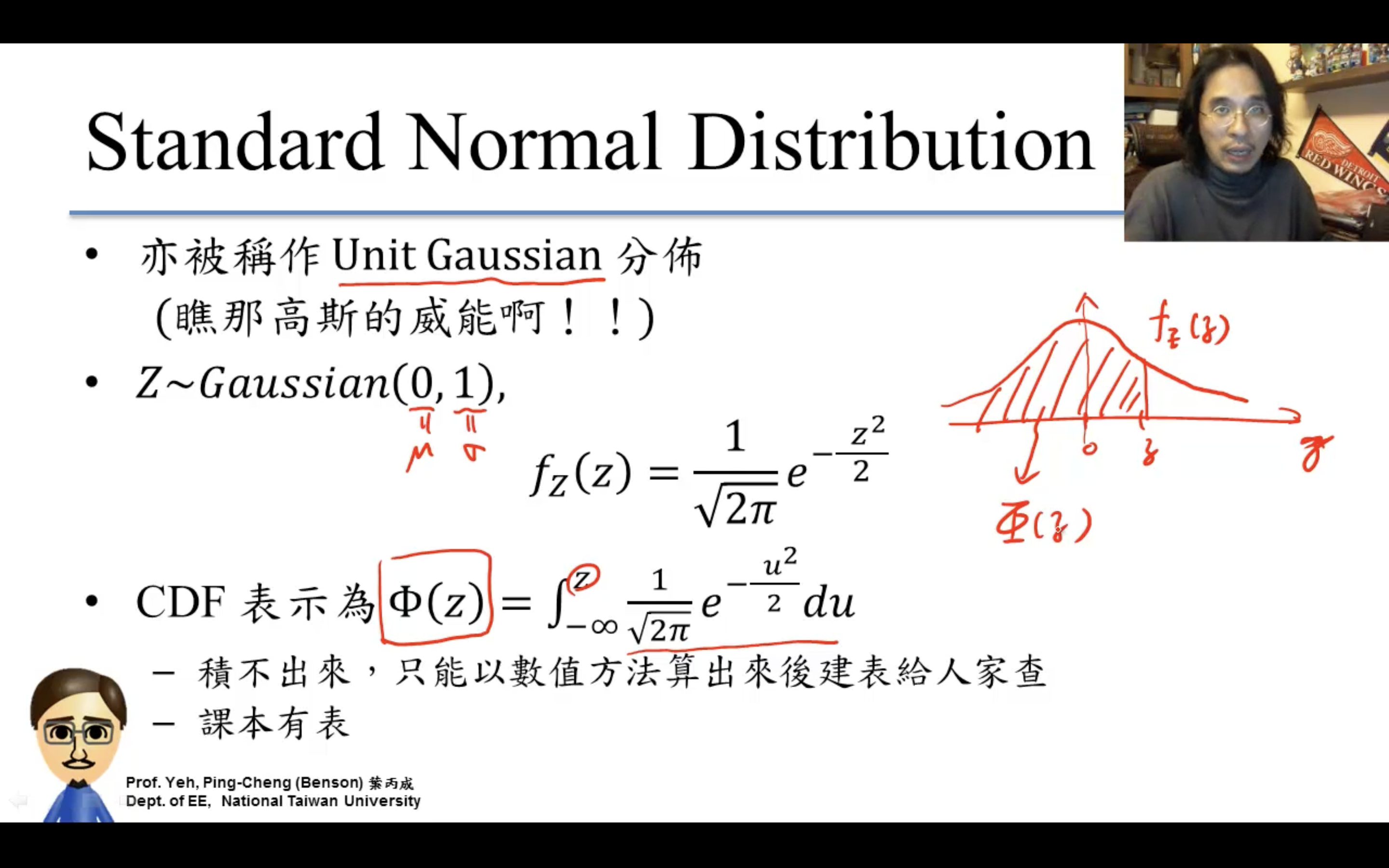
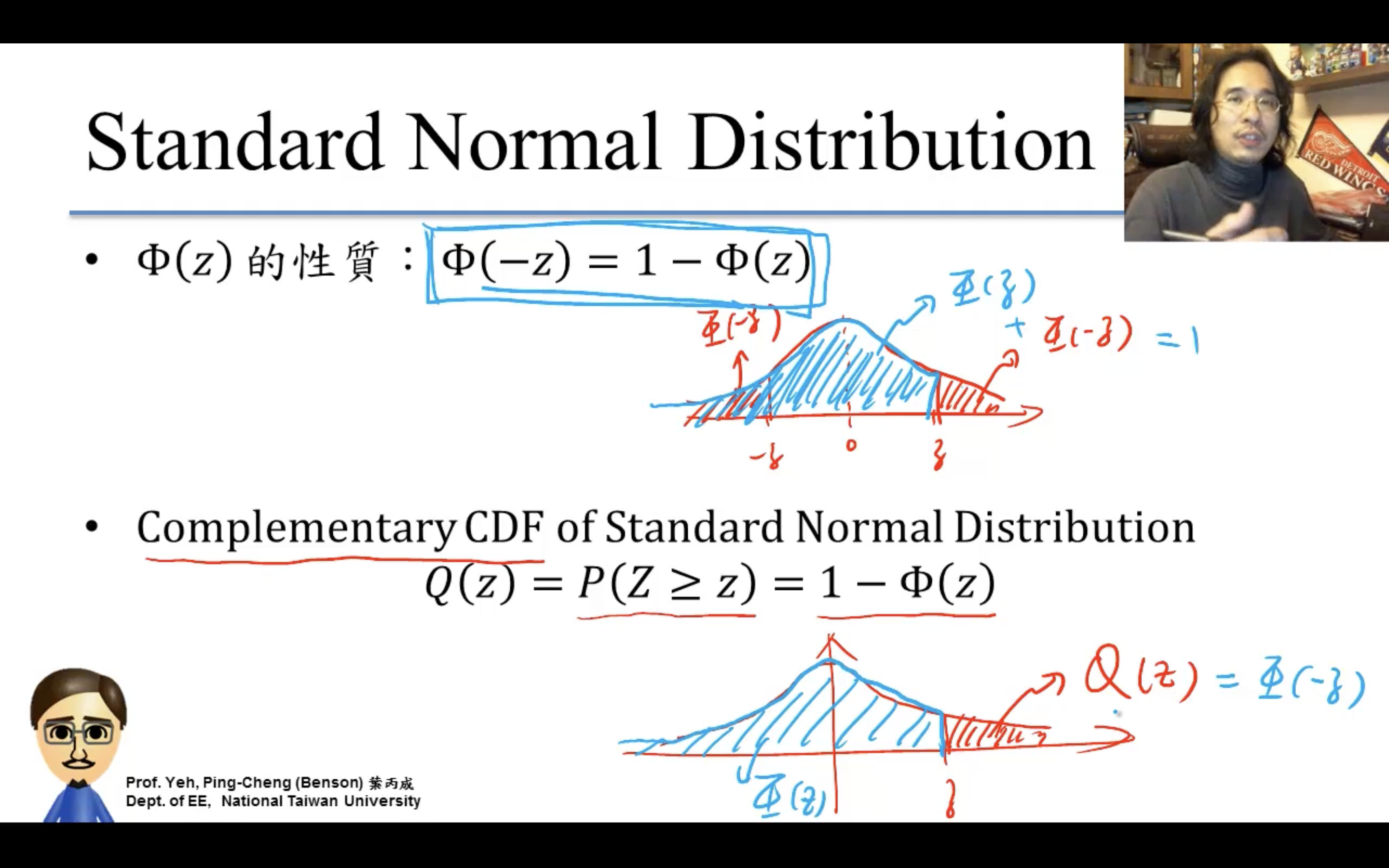
比如gaussian，為什麼單獨對standard normal建表？因為：。。。

https://en.wikipedia.org/wiki/Normal_distribution

Central Limit Theorem(中央極限定理)

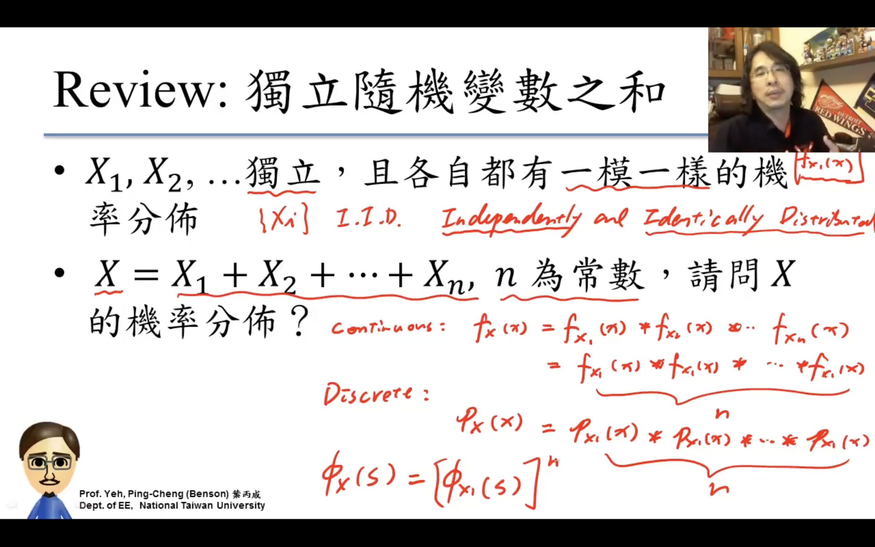
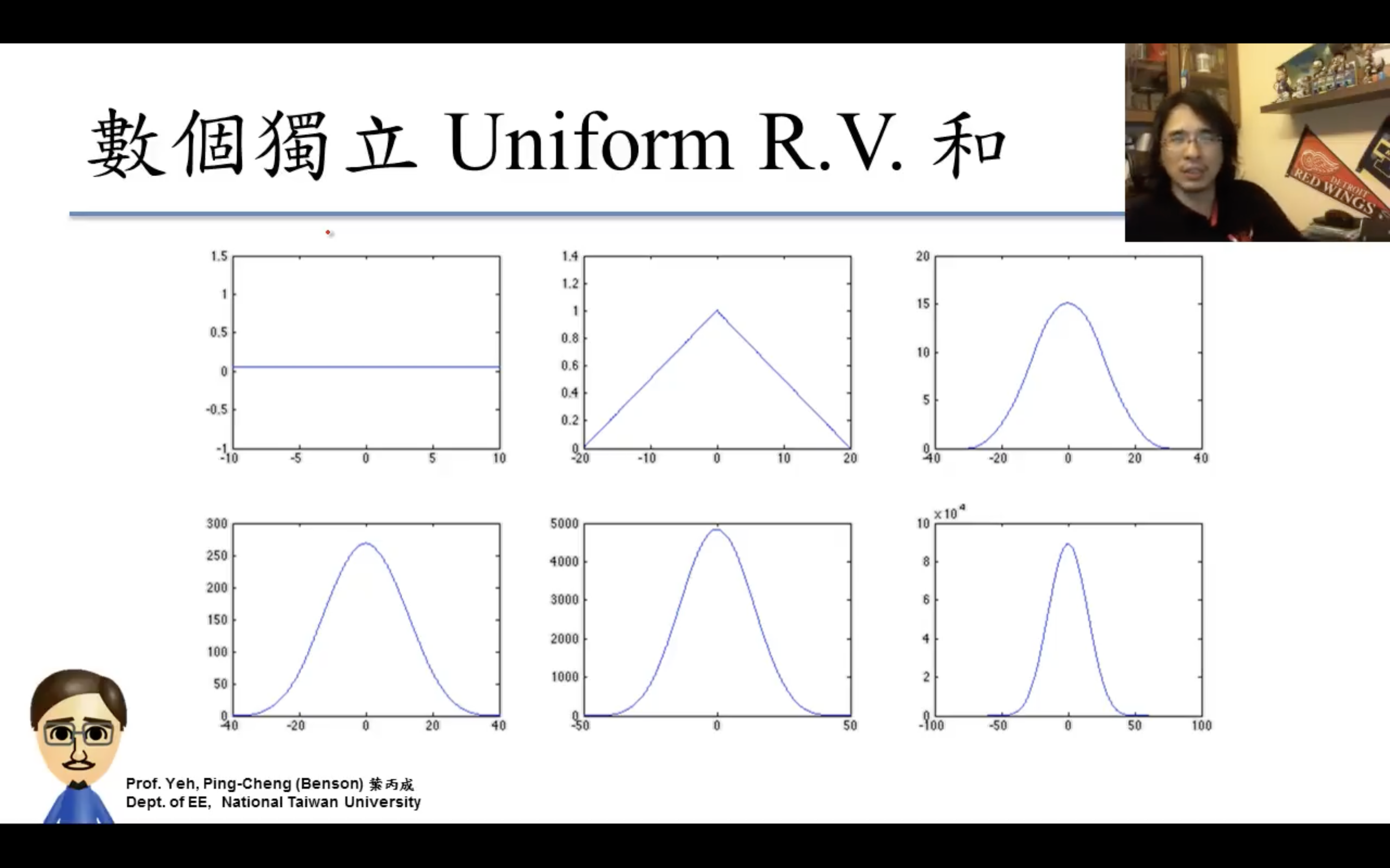
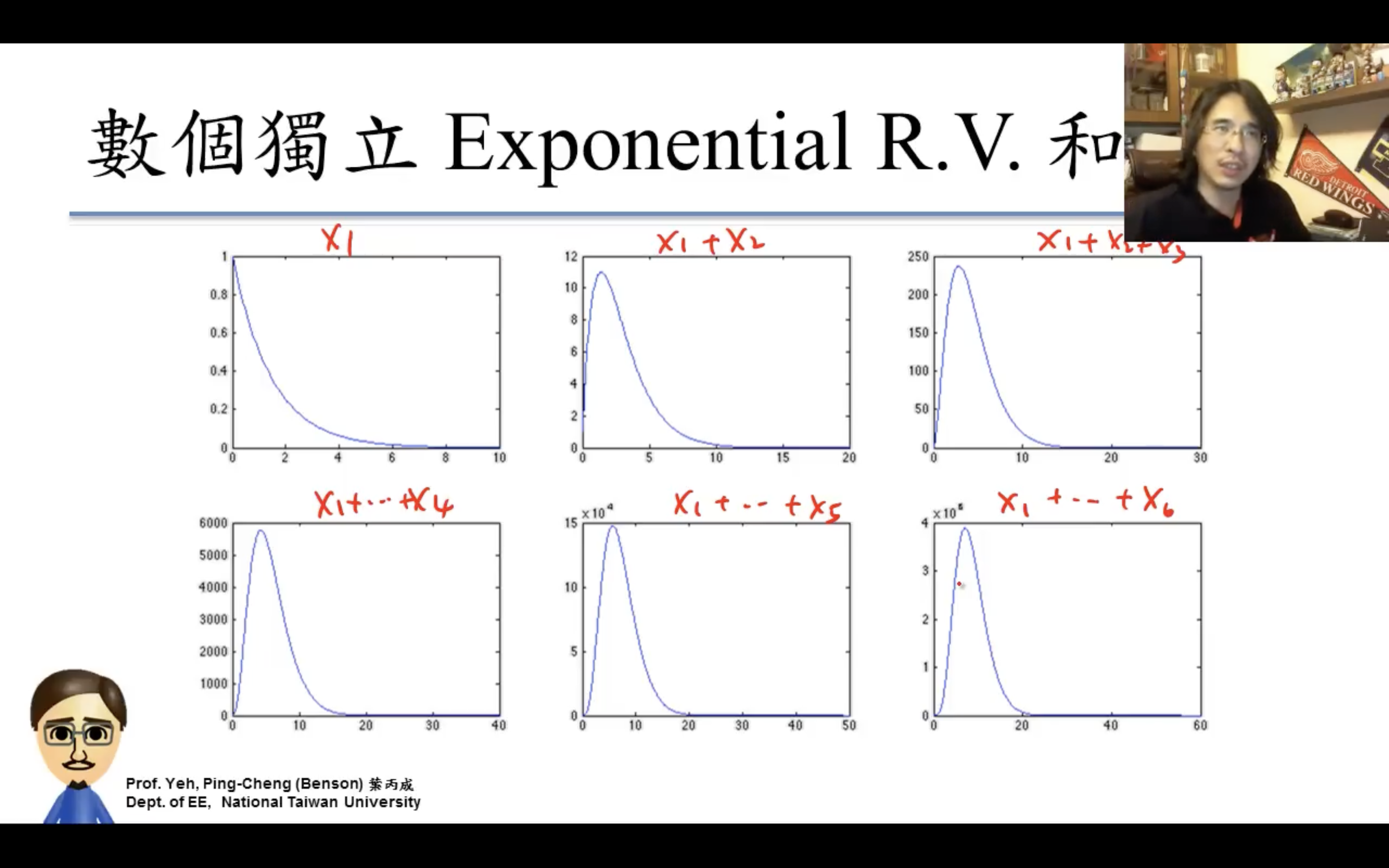
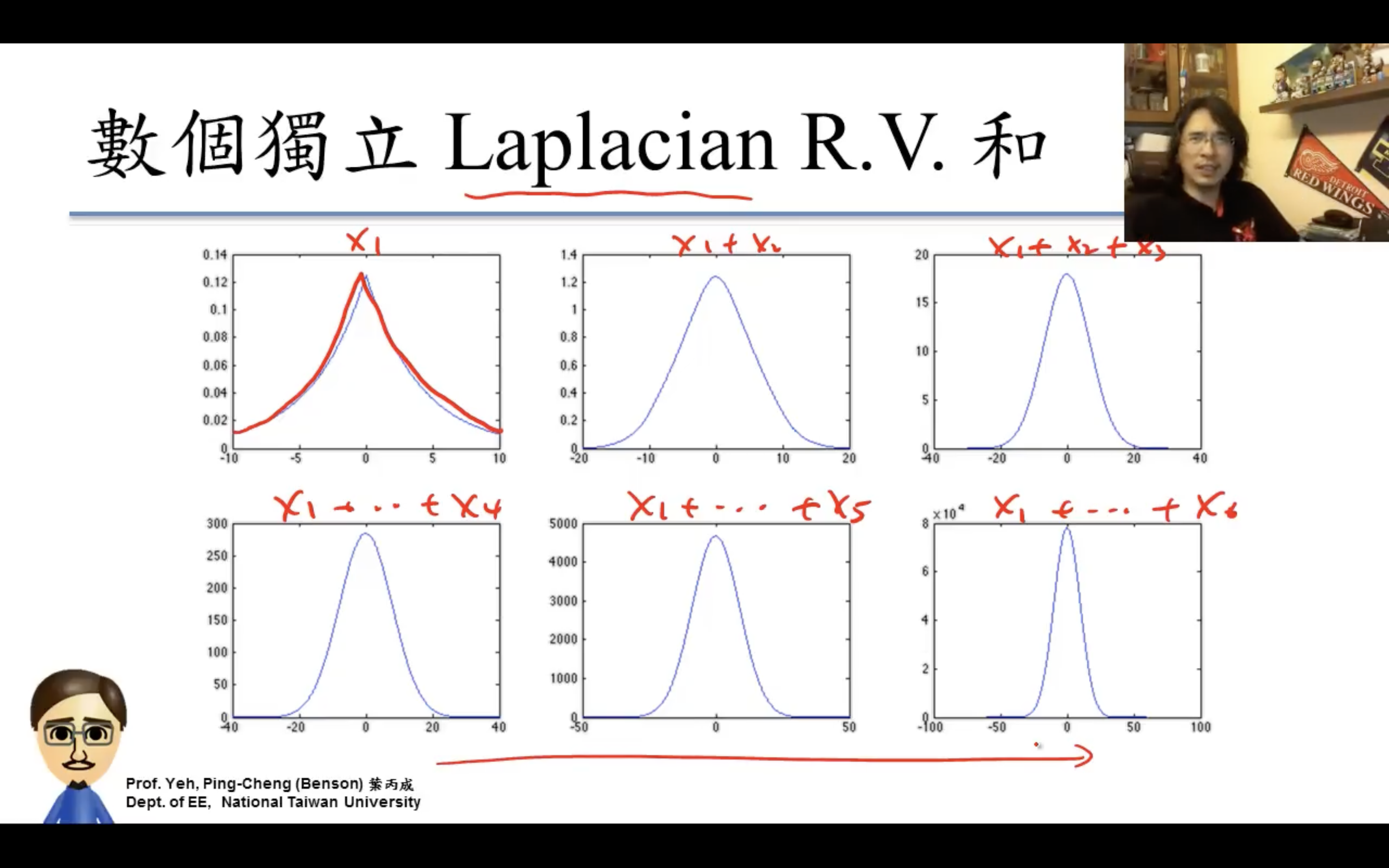
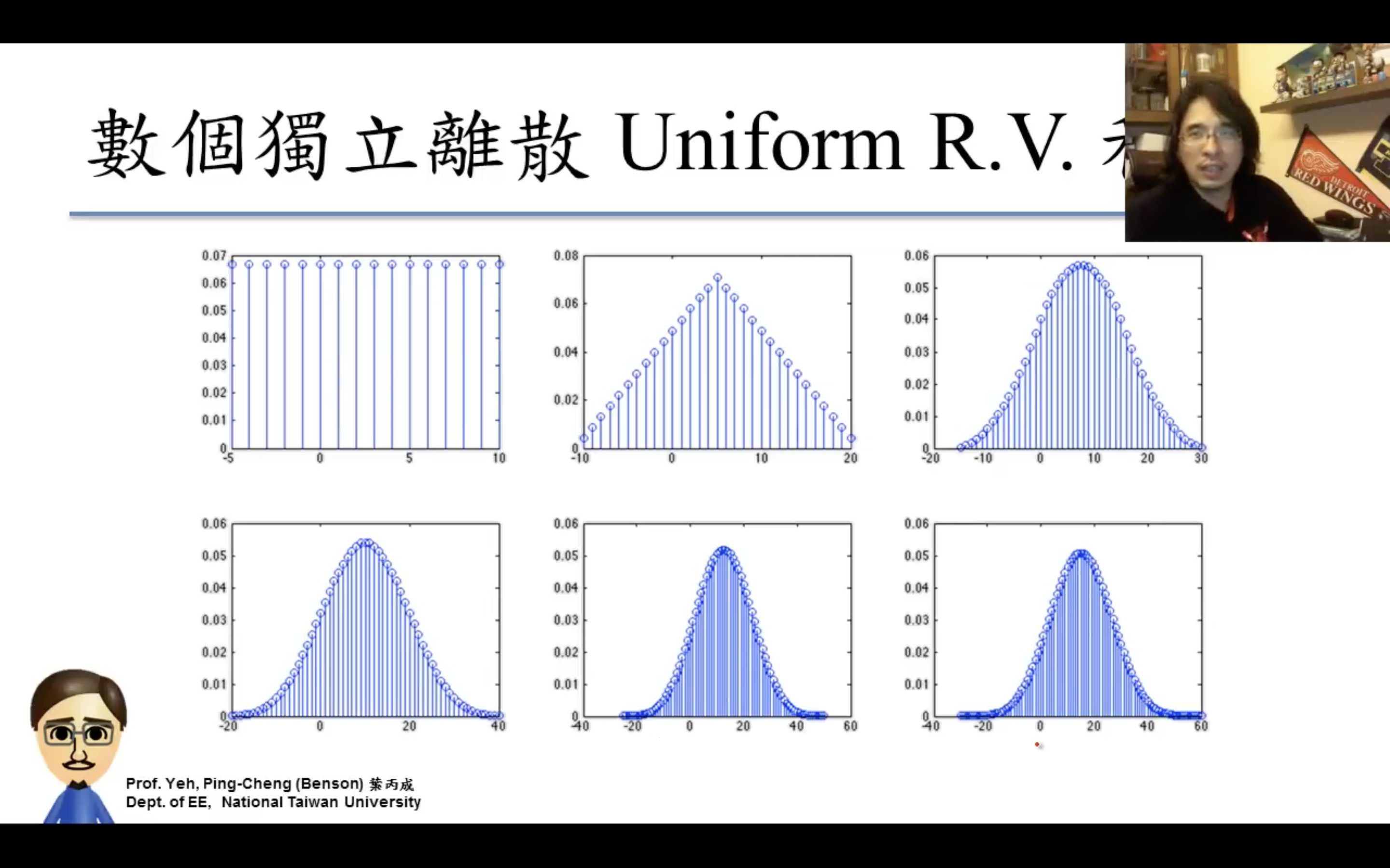
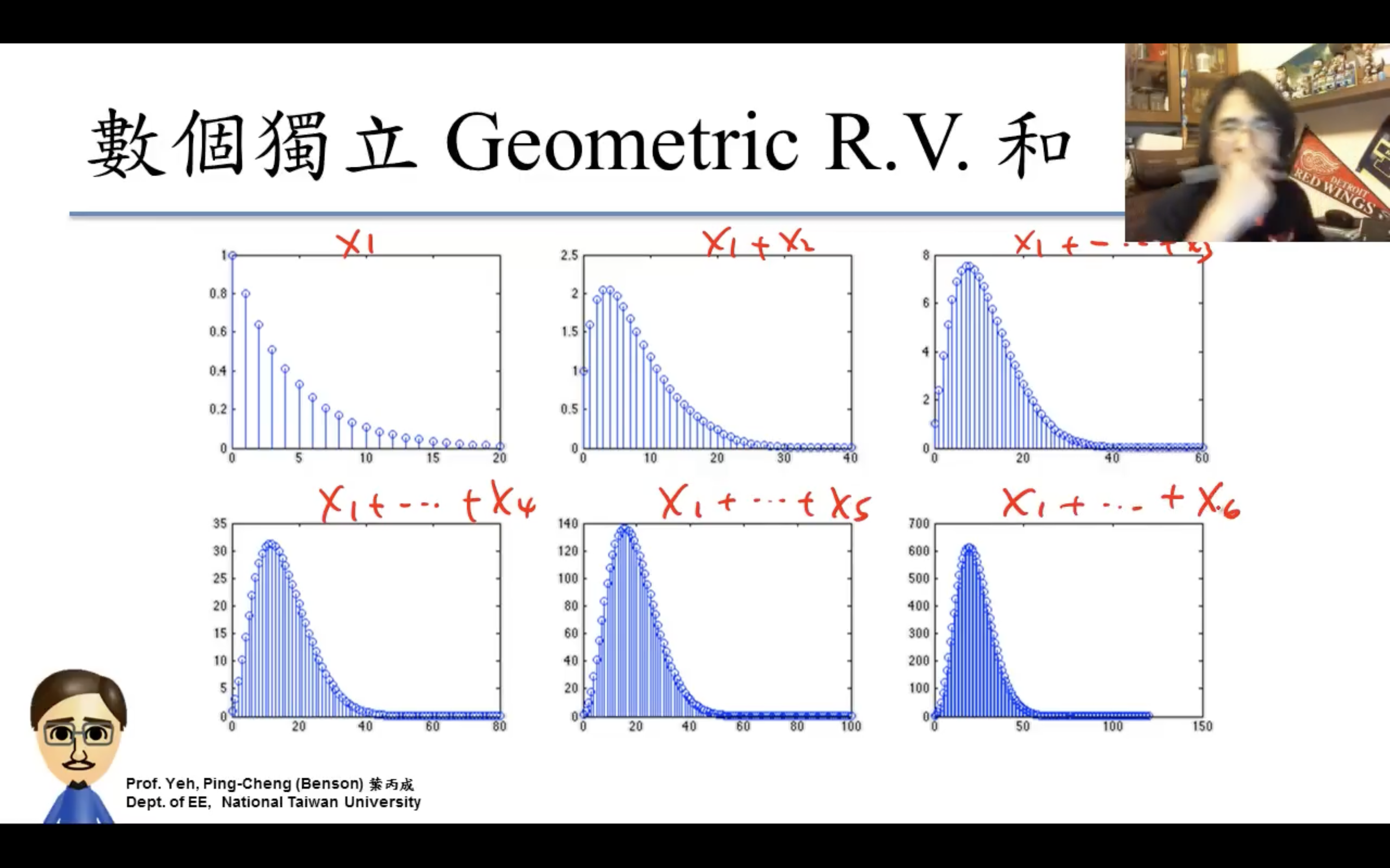
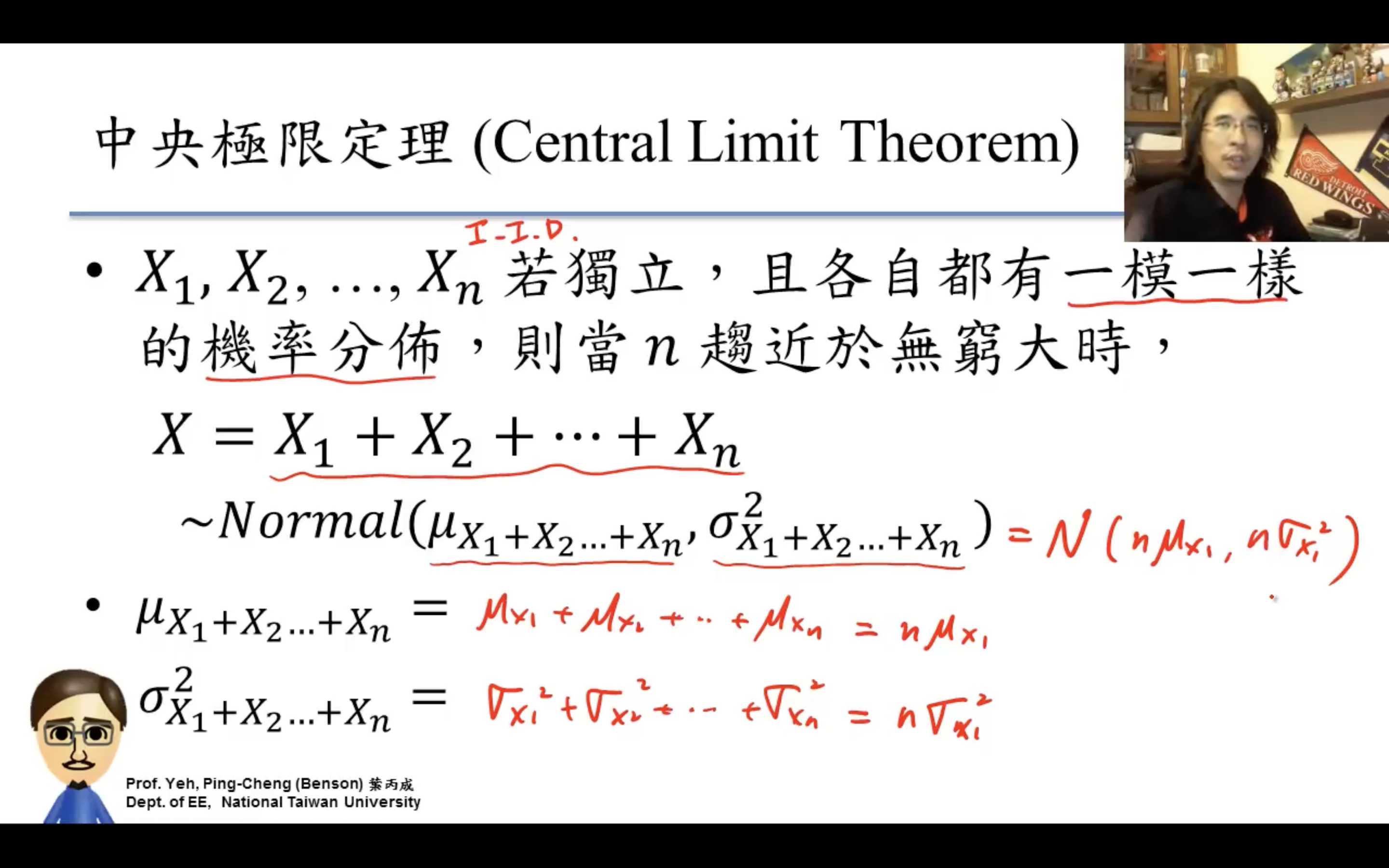
應用

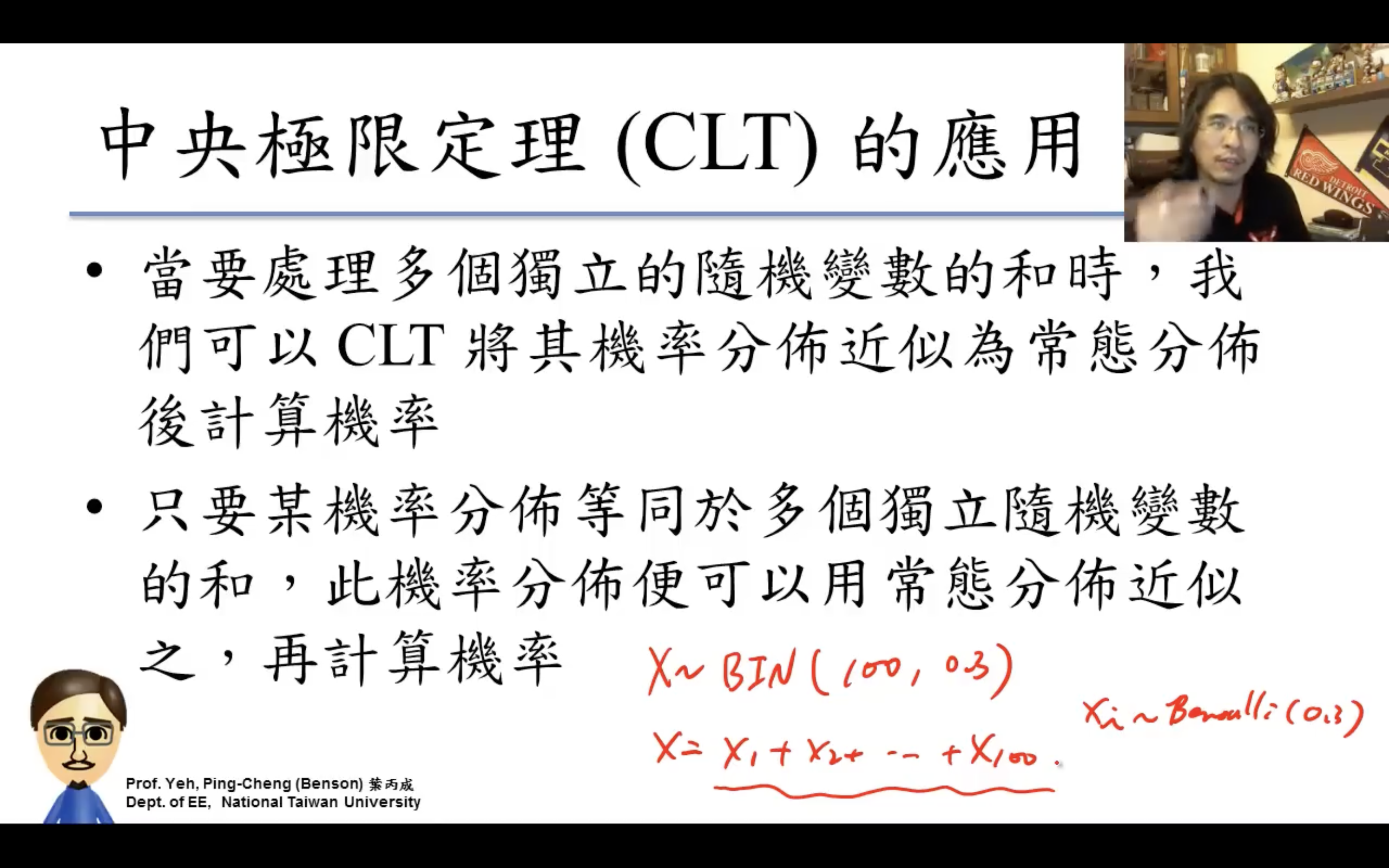
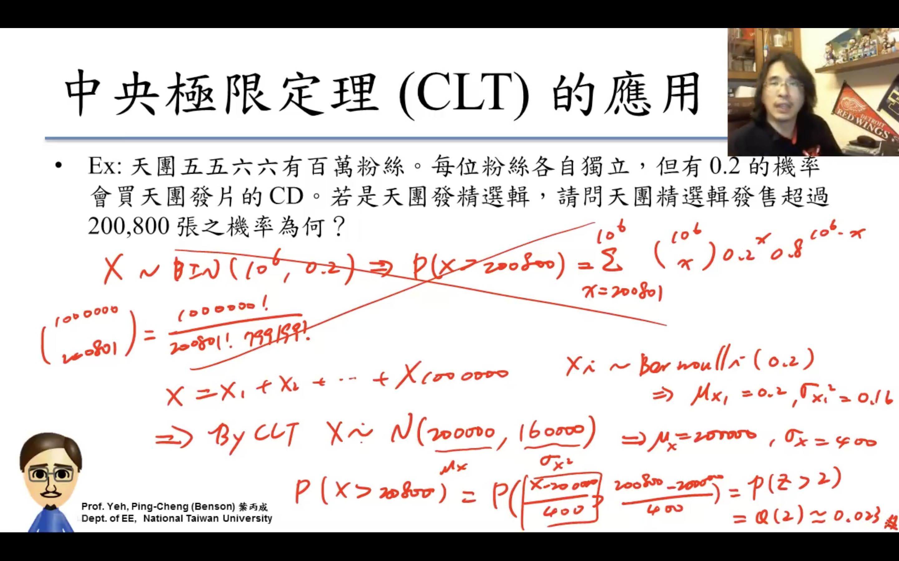
為什麼mean是probability，variance是probability(1- probability)，因為Bernoulli的X非1即0，所以expectation是1*probability + 0*(1- probability)，$Var(X)=E(X^2)-E(X)^2 = probability - probability^2$。

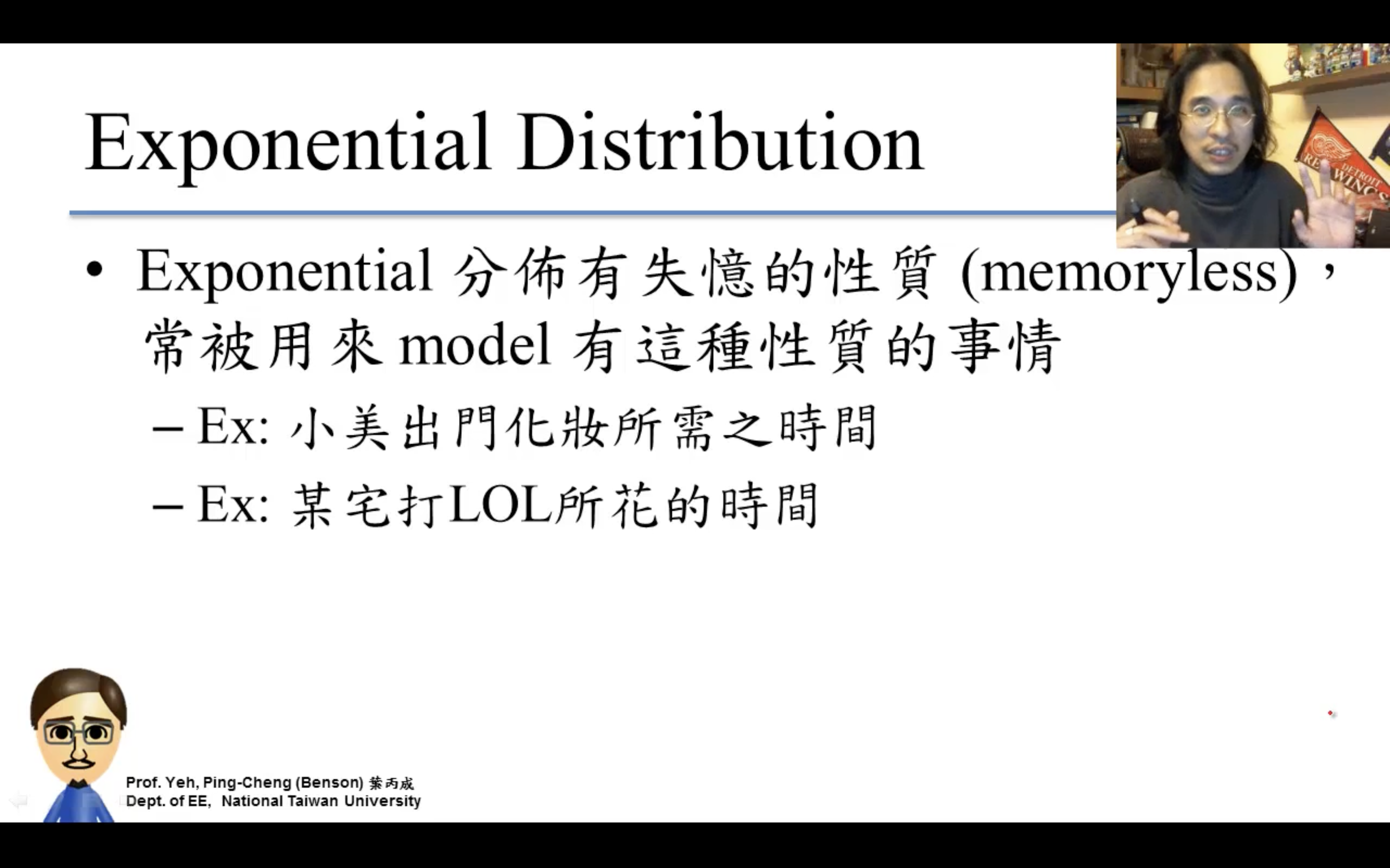
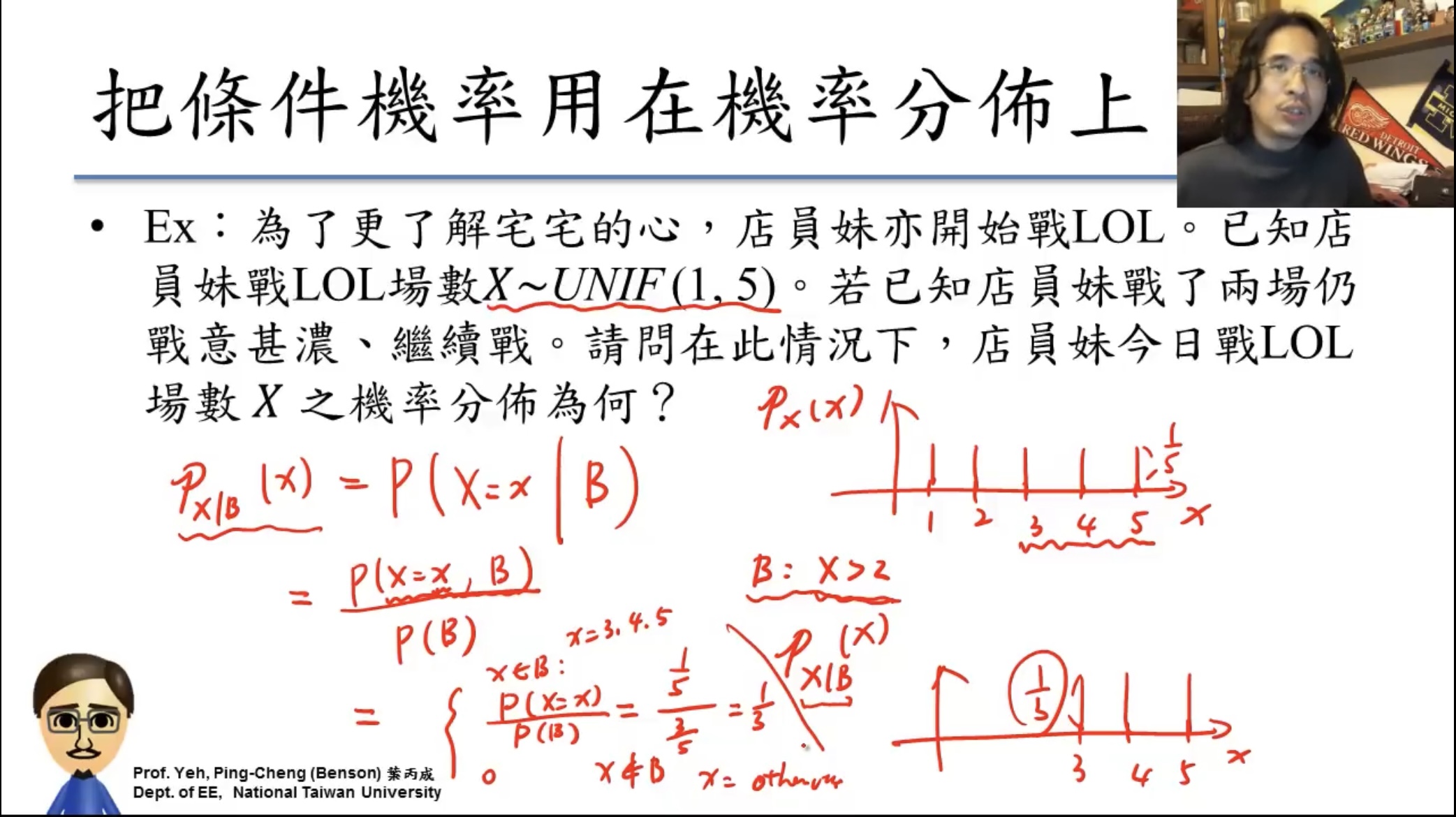
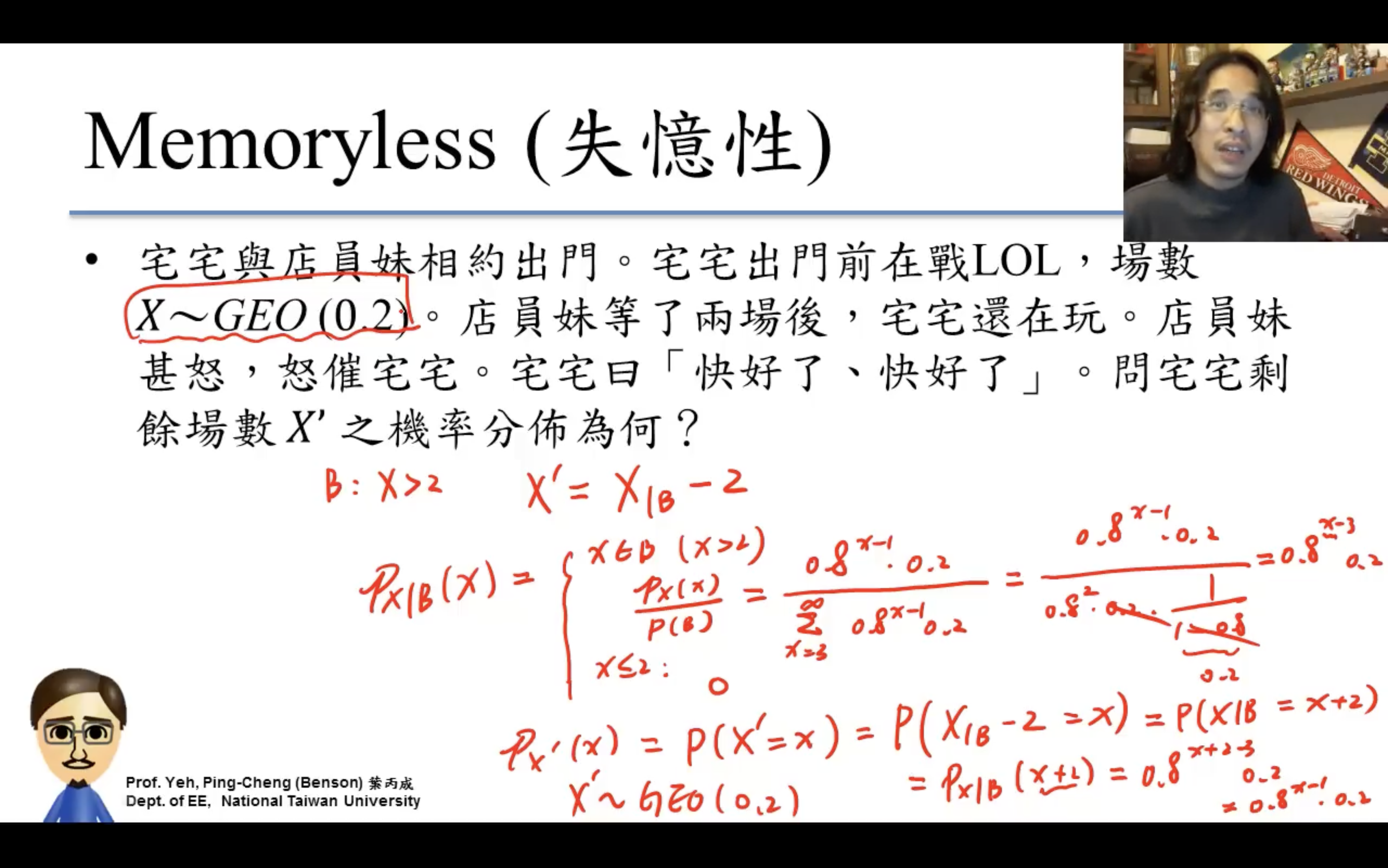
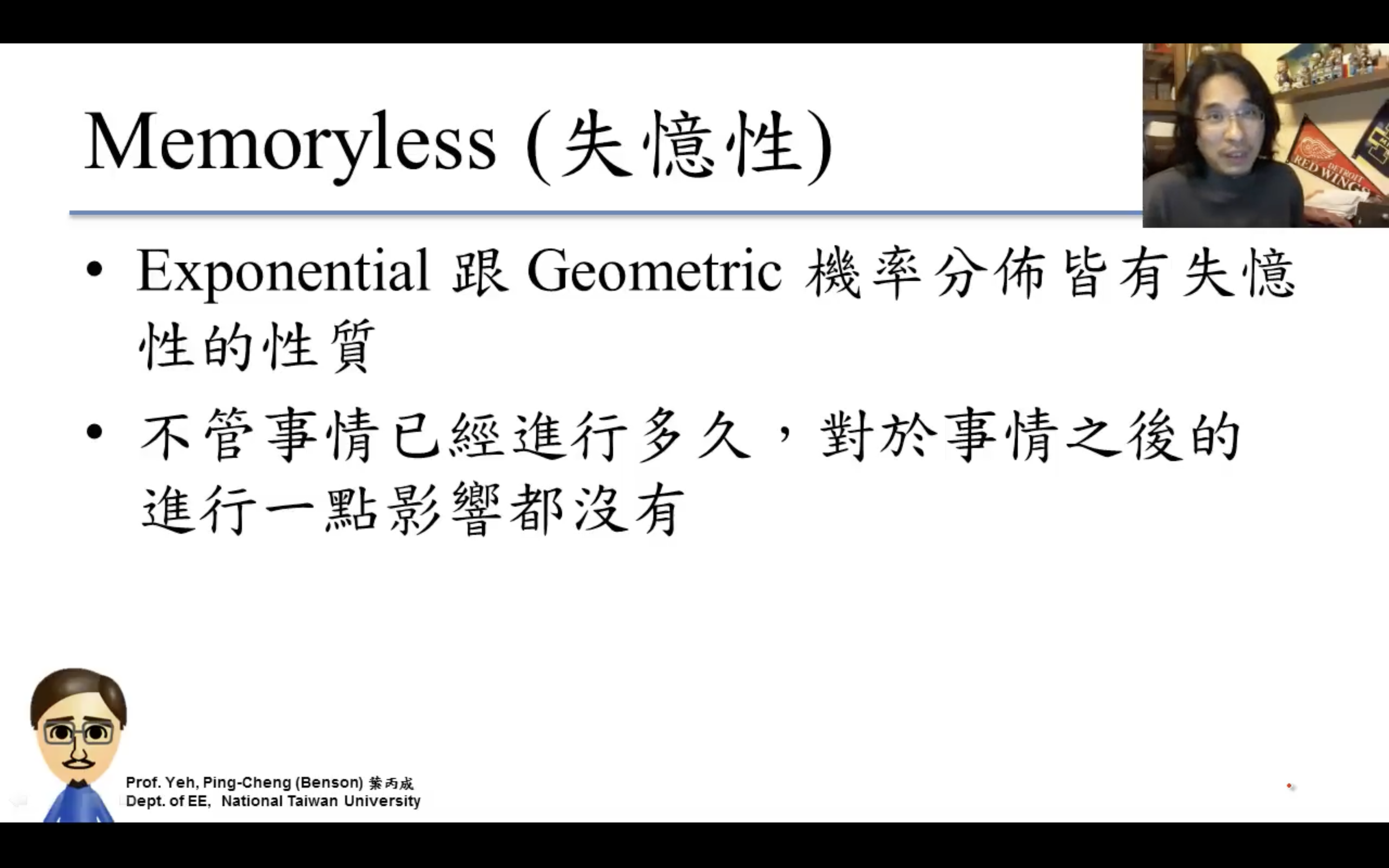
失憶性

dota mmr

https://dota2.fandom.com/wiki/Matchmaking
https://dota2.fandom.com/wiki/Matchmaking_Rating

Valve has stated that matchmaking tries to fulfil several criteria:

• The teams are balanced. (Each team has a 50% chance to win. It's based on Elo rating.)
• The discrepancy in skill between the most and least skilled player in the match is minimized.
• The highest skill Radiant player should be close to the same skill as the highest skill Dire player.
• The discrepancy between experience (measured by the number of games played) between the least experienced player and the most experienced player is minimized.
• Each team contains about the same number of parties.
• Five-player parties can only be matched against other five-player parties.
• Players' language preferences contains a common language.
• Wait times shouldn't be too long.

elo hell

Elo hell (also known as MMR hell) is a video gaming term used in MOBAs and other multiplayer online games with competitive modes. It refers to portions of the matchmaking ranking spectrum where individual matches are of poor quality, and are often determined by factors such as poor team coordination which are perceived to be outside the individual player's control. This ostensibly makes it difficult for skilled players to "climb" up the matchmaking ranking (and out of Elo hell), due to the difficulty of consistently winning games under these conditions. Its existence in various games has been debated, and some game developers have called it an illusion caused by cognitive bias.

在北街咖啡斷網的瞬間記起小時候爸帶回家一台筆記本電腦，那時上網還通通都是有線和sim卡，而那台筆記本是插無線網卡上網。在老家屬院那間客廳的衣櫥上用插著一根錄音筆一樣的無線網卡的筆記本電腦玩賽爾號（打普尼？），那真是堪比幾年後我用小手機看網路小說到天亮，爸第二天在我確定他沒有翻我手機的情況下能精準說出我瀏覽了哪些網頁一樣的震撼體驗。這一幕幕歷歷在目。